

Opinions. Are they positive or negative?
Opinion mining has attracted great interest in recent years. One of the most promising applications is analysis of opinions in social networks. Opinion mining in a broad sense is defined as the computational study of opinions, sentiments and emotions expressed in texts.
Following the series of videos from Paeng Angnakoon I try to do the same. However once I applied the code for twits in Spanish the output was none because the lexicons were in English. After some Google searches I found the Spanish lexicons from Veronica Perez Rosas, Carmen Banea, Rada Mihalcea which I adapted to fit the package sentiment, which by the way does not work under the version 3 of R. So the solution was to convert the package to functions. The package sentiment use a naive Bayes as categorizer engine. In a recent email Carmen Baena suggested me to use Weka. apparently it is a very robust machine learning suite. I hope to find the time to give it a try. Another lexicom I am using here is from Grigori SIDOROV.
My Example
I wanted to investigate the opinions in twitter for Cucuta, my town. Also for Santurban a polemic region were gold mining is colliding with Paramo conservation, and the Catatumbo region another complex and even dangerous place in Norte de Santander, Colombia. In Catatumbo coca cultivation, African palm cultivation, guerrillas, paramilitary groups, Colombian army and corruption have made an explosive cocktail.
Get the code from my Github
To follow the code first get twitter access from R
Paeng Angnakoon explain it very well in her first video.
library(twitteR)
library(ROAuth)
library(plyr)
library(stringr)
library(ggplot2)
library(tm)
## Windows users need to get this file
download.file(url="http://curl.haxx.se/ca/cacert.pem", destfile="cacert.pem")

requestURL <- "https://api.twitter.com/oauth/request_token"
accessURL = "https://api.twitter.com/oauth/access_token"
authURL = "https://api.twitter.com/oauth/authorize"
consumerKey = "XXXXXXXXXXXXXXXXXXXXXXXXX" # use yours
consumerSecret = "XXXXXXXXXXXXXXXXXXXXXXXXXX" # use yours
Cred <- OAuthFactory$new(consumerKey=consumerKey,
                         consumerSecret=consumerSecret,
                         requestURL=requestURL,
                         accessURL=accessURL,
                         authURL=authURL)
Cred$handshake(cainfo = system.file("CurlSSL", "cacert.pem", package = "RCurl") )
6235667
save(Cred, file="twitter authentication.Rdata")
registerTwitterOAuth(Cred)
## Future use
load("twitter authentication.Rdata")
registerTwitterOAuth(Cred)
Twitter scrape #Catatumbo #SanTurban #Cucuta
Catatumbo.list <- searchTwitter('Catatumbo', n=1000, cainfo="cacert.pem")
Catatumbo.df = twListToDF(Catatumbo.list)
write.csv(Catatumbo.df, file='C:/temp/CatatumboTweets.csv', row.names=F)

SanTurban.list <- searchTwitter('Santurban', n=1000, cainfo="cacert.pem", since='2010-03-01')
SanTurban.df = twListToDF(SanTurban.list)
write.csv(SanTurban.df, file='C:/temp/SanTurbanTweets.csv', row.names=F)

Cucuta.list <- searchTwitter('Cucuta', n=1000, cainfo="cacert.pem")
Cucuta.df = twListToDF(Cucuta.list)
write.csv(Cucuta.df, file='C:/temp/CucutaTweets.csv', row.names=F)
Loading emotion, polarity and score.sentiment functions
source("classify_polarity.R")
source("classify_emotion.R")
source("create_matrix.R")

score.sentiment = function(sentences, pos.words, neg.words, .progress='none')
{
  require(plyr)
  require(stringr)
  # we got a vector of sentences. plyr will handle a list
  # or a vector as an "l" for us
  # we want a simple array ("a") of scores back, so we use
  # "l" + "a" + "ply" = "laply":
  scores = laply(sentences, function(sentence, pos.words, neg.words) {
    # clean up sentences with R's regex-driven global substitute, gsub():
    sentence = gsub('[[:punct:]]', '', sentence)
    sentence = gsub('[[:cntrl:]]', '', sentence)
    sentence = gsub('\\d+', '', sentence)
    # and convert to lower case:
    sentence = tolower(sentence)
    # split into words. str_split is in the stringr package
    word.list = str_split(sentence, '\\s+')
    # sometimes a list() is one level of hierarchy too much
    words = unlist(word.list)
    # compare our words to the dictionaries of positive & negative terms
    pos.matches = match(words, pos.words)
    neg.matches = match(words, neg.words)
    # match() returns the position of the matched term or NA
    # we just want a TRUE/FALSE:
    pos.matches = !is.na(pos.matches)
    neg.matches = !is.na(neg.matches)
    # and conveniently enough, TRUE/FALSE will be treated as 1/0 by sum():
    score = sum(pos.matches) - sum(neg.matches)
    return(score)
  }, pos.words, neg.words, .progress=.progress )
  scores.df = data.frame(score=scores, text=sentences)
  return(scores.df)
}
Some scores
Catatumbo.scores = score.sentiment(DatasetCatatumbo$text, pos.words,neg.words, .progress='text')
SanTurban.scores = score.sentiment(DatasetSanTurban$text, pos.words,neg.words, .progress='text')
Cucuta.scores = score.sentiment(DatasetCucuta$text, pos.words,neg.words, .progress='text')

Catatumbo.scores$Team = 'Catatumbo'
SanTurban.scores$Team = 'SanTurban'
Cucuta.scores$Team = 'Cucuta'
Make the graph comparing the 3 data sets
all.scores = rbind(Catatumbo.scores, SanTurban.scores, Cucuta.scores)
ggplot(data=all.scores) + # ggplot works on data.frames, always
  geom_bar(mapping=aes(x=score, fill=Team), binwidth=1) +
  facet_grid(Team~.) + # make a separate plot for each hashtag
  theme_bw() + scale_fill_brewer() # plain display, nicer colors
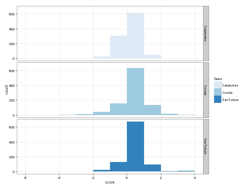
It is interesting to see how Catatumbo has the worst score and Santurban some few really high scores >3.
What about Santurban?
According to a prominent biodiversity guru in Colombia and the high-lines of a newspaper, Santurban polarized the country. So I wanted to describe the Santurban opinions in twitter in a systematic way.
# first some processing
SanTurban_txt = sapply(SanTurban.list, function(x) x$getText())
# Prepare text for the analysis
SanTurban_txt = gsub("(RT|via)((?:\\b\\W*@\\w+)+)", "", SanTurban_txt)
SanTurban_txt = gsub("@\\w+", "", SanTurban_txt)
SanTurban_txt = gsub("[[:punct:]]", "", SanTurban_txt)
SanTurban_txt = gsub("[[:digit:]]", "", SanTurban_txt)
SanTurban_txt = gsub("http\\w+", "", SanTurban_txt)
SanTurban_txt = gsub("[ \t]{2,}", "", SanTurban_txt)
SanTurban_txt = gsub("^\\s+|\\s+$", "", SanTurban_txt)

try.error = function(x){
  # create missing value
  y = NA
  # tryCatch error
  try_error = tryCatch(tolower(x), error=function(e) e)
  # if not an error
  if (!inherits(try_error, "error"))
    y = tolower(x)
  # result
  return(y)
}
# lower case using try.error with sapply
SanTurban_txt = sapply(SanTurban_txt, try.error)
# remove NAs in SanTurban_txt
SanTurban_txt = SanTurban_txt[!is.na(SanTurban_txt)]
names(SanTurban_txt) = NULL
#classify emotion
class_emo = classify_emotion(SanTurban_txt, algorithm="bayes", prior=1.0)
#get emotion best fit
emotion = class_emo[,7]
# substitute NA's by "unknown"
emotion[is.na(emotion)] = "unknown"
# classify polarity
class_pol = classify_polarity(SanTurban_txt, algorithm="bayes")
# get polarity best fit
polarity = class_pol[,4]
# data frame with results
sent_df = data.frame(text=SanTurban_txt, emotion=emotion,
                     polarity=polarity, stringsAsFactors=FALSE)
# sort data frame
sent_df = within(sent_df,
             emotion <- factor(emotion, levels=names(sort(table(emotion), decreasing=TRUE))))
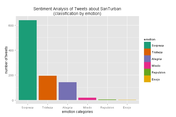
Now the graphs
# plot distribution of emotions
ggplot(sent_df, aes(x=emotion)) +
  geom_bar(aes(y=..count.., fill=emotion)) +
  scale_fill_brewer(palette="Dark2") +
  labs(x="emotion categories", y="number of tweets",
       title = "Sentiment Analysis of Tweets about SanTurban\n(classification by emotion)",
       plot.title = element_text(size=12))

# plot distribution of polarity
ggplot(sent_df, aes(x=polarity)) +
  geom_bar(aes(y=..count.., fill=polarity)) +
  scale_fill_brewer(palette="RdGy") +
  labs(x="polarity categories", y="number of tweets",
       title = "Sentiment Analysis of Tweets about SanTurban\n(classification by polarity)",
       plot.title = element_text(size=12))
- First by Emotion
- Next by Polarity
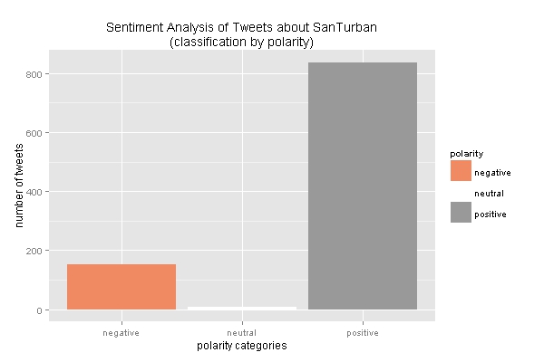
It is Clear:
- Most of Santurban opinions are positive. I guess they are coming from the government agencies. Or is the Bayesian classifier skew to positive scores?
- The country is not polarized at all. At least in twitter the positive opinions are more frequent.

This work is licensed under a Creative Commons Attribution-ShareAlike 4.0 International License.