

Mammal records in Colombia
Disappointed by the last report of Colombia to the CBD that does not mention how much Colombia knows about its biodiversity, I decided to carry out a basic analysis using mammal data and R.
In my opinion the report is only focused on ecosystem services and biodiversity loss is only mentioned as an impact of deforestation. But my opinion on this matter will be the subject of another post.
My Example
First, I downloaded the mammal data set for Colombia from GBIF, which you can get here. The data set has 85318 records (probably more if you get it after May 2014). From those records I selected those with hard evidence, i.e., the ones having preserved specimens, eliminating 1893 observations, mainly from iNaturalist and Corantioquia.
Some georeferences were really wrongly made, plotting points outside Colombia. So I decided to overwrite those coordinates using NAs. At the end I used only 36031 georeferenced points, less than half of the total data set, to generate maps. It is sad to discover that more than half of the records are wrong or not georeferenced.
Before making the maps I fixed some issues, such as empty records and the 8200001422-01 problem, which you can see in detail at the end of this post.
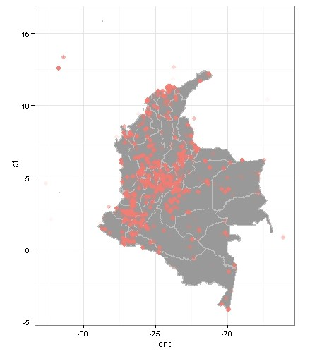
Plotting all the records, the map looks like this:
require(ggmap)
require(raster)
require(plyr)

bigtable<-read.csv(file="data\\GBIF\\occurrenceGBIF_Mammal.txt",header=T,sep="\t")
bigtable<-subset(bigtable, basisofrecord=="PRESERVED_SPECIMEN") #only collected specimens

#get poligon of Colombia
co<-getData("GADM",country="CO",level=1,download=TRUE)
col_depto <- fortify(co,region="NAME_1") # make compatible to ggplot2

mapbase<- ggplot(col_depto, aes(long,lat,group=group)) +
	geom_polygon(fill="grey60") + coord_equal() +
	geom_path(color="grey")

delet<-which(x=bigtable$decimallongitude> -66) #select points way outside Colombia
bigtable[delet,79]<-NA
bigtable[delet,80]<-NA
delet<-which(x=bigtable$decimallongitude< -83) #select points way outside Colombia
bigtable[delet,79]<-NA
bigtable[delet,80]<-NA
delet<-which(x=bigtable$decimallatitude> 14) #select points way outside Colombia
bigtable[delet,79]<-NA
bigtable[delet,80]<-NA
delet<-which(x=bigtable$decimallatitude< -5) #select points way outside Colombia
bigtable[delet,79]<-NA
bigtable[delet,80]<-NA

# fix empty values in publishingcountry <- empty are colombian
nada<-which(x=bigtable$publishingcountry=="")
bigtable$publishingcountry[nada]<-"CO"
# make a new category Colombia Vs International
CO<-which(x=bigtable$publishingcountry=="CO")
bigtable$int_col<-"International"
bigtable$int_col[CO]<-"Colombia"
# fix 8200001422-01 problem. See http://tapirologist.wordpress.com/2013/06/04/biodiversity-by-colombian-institutions/
Iavh<-which(x=bigtable$institutioncode=="8200001422-01")
bigtable$institutioncode[Iavh]<-"IAvH"

## mapping all points
map1<-mapbase + geom_point(aes(x = decimallongitude, y = decimallatitude, group = TRUE,
                      colour = "red"),
                      data = bigtable, size = 3,
                      alpha = 1/15) +
                      theme_bw() + guides(guide_legend((title = NULL)))+
                      theme(legend.position = "none")
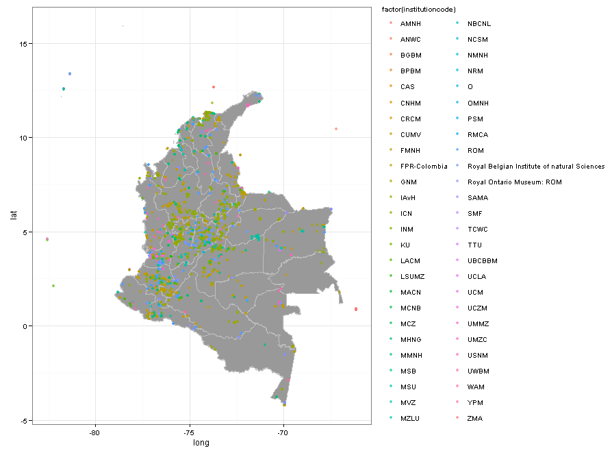
Adding colors by collection, the map looks like this.
### mapping all mammal collections for Col in GBIF
map2<-mapbase + geom_point(aes(x = decimallongitude, y = decimallatitude, group = TRUE,
                          colour = factor(institutioncode)),
                          data = bigtable, size = 2,
                          alpha=2/3) +
  theme(legend.position = "right") +
  theme_bw() + guides(col = guide_legend(ncol = 2)) +
  theme(legend.key = element_rect(colour = "white"))
There are some problems. ROM is duplicated and there are weird institutions such as “O”. But overall you can see that the only Colombian institutions reporting mammals to GBIF are ICN and IAvH. It is sad that other large mammal collections such as Universidad del Valle, Universidad de Antioquia, Universidad del Cauca, and Universidad Javeriana are not reporting data to GBIF.
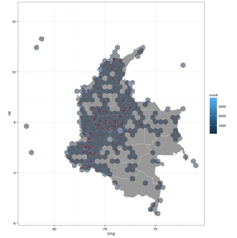
Adding a hexagon of approx 100 km around each collection point we can discover places undersampled in mammal collections
#### Were have been collected the mammals
map3<-mapbase + geom_point(aes(x = decimallongitude, y = decimallatitude, group = FALSE), size=1,
                           data = bigtable,alpha=I(0.25),colour="red") +
  stat_binhex(aes(x = decimallongitude, y = decimallatitude, group = FALSE),
              size = .5, binwidth = c(.5,.5), alpha = 2/4,data = bigtable) + theme_bw()
What about contrasting Colombian institutions against other foreign ones?
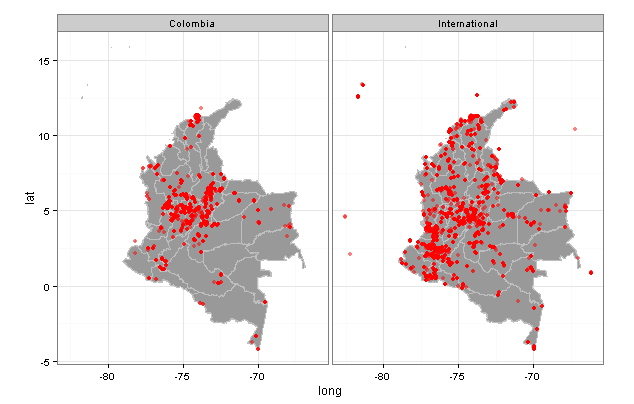
Well the places were mammals have been collected by Colombian institutions are fewer.
##### Colombia vs International
map4<-mapbase + geom_point(aes(x = decimallongitude, y = decimallatitude, group = FALSE), size=2,
                           data = bigtable,alpha=I(0.5),colour="red") +
                          facet_wrap(~ int_col) + theme_bw()
Which are those international countries and what kind of mammals do they have?
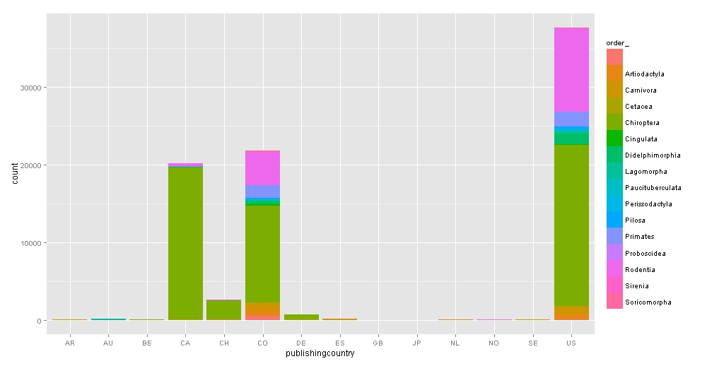
Bats are the most popular species in collections and the US is the winner.
### bar graph by country and order collected
barcountry<-ggplot(bigtable, aes(publishingcountry, fill=order_)) +
  geom_bar() + scale_colour_brewer(palette="Set1")
What about if we ask for the years of collection?

The records start before 1800 and end in 2006. Interesting: There is a big peak in 1967.
Unfortunately that huge collection peak do not correspond to a Colombian institution.
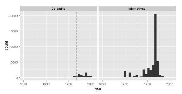
The big contribution from 1967 was for the USNM and the ROM

The doted red line is the year 1967.
count<-ddply(bigtable,.(year), summarize, freq=length(year))
count<-count[2:120,] # ignore 1700

colectime<-ggplot(count, aes(x=year, y=freq, xmin=1800)) + geom_line() +
  geom_vline(xintercept = 1967,colour="red", linetype = "longdash") +
  annotate("text", label = "1967", x = 1967, y = 6900, size = 5, colour = "blue")

ggplot(bigtable, aes(year)) + geom_bar() + xlim(1850, 2006) +
  geom_vline(xintercept = 1967,colour="red", linetype = "longdash")+
  facet_wrap(~ int_col)

ggplot(bigtable, aes(year)) + geom_bar() + xlim(1850, 2006) +
  geom_vline(xintercept = 1967,colour="red", linetype = "longdash")+
  facet_wrap(~ institutioncode,nrow = 10)
So what happened in 1967?
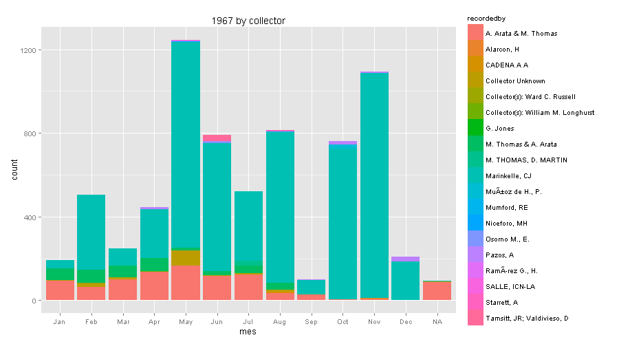
The great professor Cornelis J. Marinkelle from Universidad de los Andes in Bogota, was very active collecting bats. Probably searching for parasites. Now I regret that I never took his class while I was a Biology student at Universidad de los Andes.
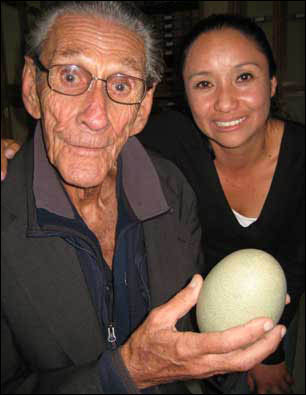
He was also an avid bird egg collector. Here’s a note from BBC mundo about him.
data1967<-subset(bigtable, year=="1967") # subset of that year
require(lubridate)
data1967$mes<-month(data1967$month,label=TRUE)
ggplot(data1967, aes(mes, fill=recordedby)) +
geom_bar() + scale_colour_brewer(palette="Set1") + ggtitle("1967 by collector")
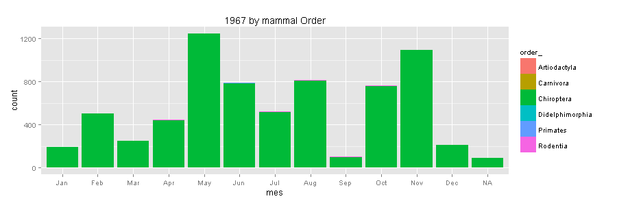
ggplot(data1967, aes(mes, fill=order_)) +
geom_bar() + scale_colour_brewer(palette="Set1") + ggtitle("1967 by mammal Order")
Amaze by the numbers I went back to the whole data set and tried to reconstruct in a map the places were Cornelis J. Marinkelle went to collect mammals. Unfortunately some years such as 1961 and 1971 do not have georeferenced records and there are a lot of georeferenced records without the year, marked as NA. I guess the data set needs a little bit more of work than a weekend.

marinkelle<-subset(bigtable, recordedby=="Marinkelle, CJ") # Just Marinkelle
map5<-mapbase + geom_point(aes(x = decimallongitude, y = decimallatitude, group = FALSE), size=2,
                           data = marinkelle,alpha=I(0.5),colour="red") +
  facet_wrap(~ year,nrow =3) + theme_bw()
The last question is why are not there more records from ICN and IAvH after 2006?
Are they not collecting any more or simply not updating their data to GBIF?
I will appreciate any comment.

This work is licensed under a Creative Commons Attribution-ShareAlike 4.0 International License.