Fitting a Spatial Factor Multi-Species Occupancy Model
Data from: Yasuni, Tamshiyacu-Tahuayo, Madidi, Plantas-Putumayo, Llanganates
model
code
analysis
453 sites, 24 mammal species
Authors
German Forero
Robert Wallace
Galo Zapara-Rios
Emiliana Isasi-Catalá
Diego J. Lizcano
Published
August 16, 2025
Single-species occupancy models
Single-species occupancy models (MacKenzie et al., 2002) are widely used in ecology to estimate and predict the spatial distribution of a species from data collected in presence–absence repeated surveys. The popularity of these models stems from their ability to estimate the effects of environmental or management covariates on species occurrences, while accounting for false-negative errors in detection, which are common in surveys of natural populations.
Multi-species occupancy models
Multi-species occupancy models for estimating the effects of environmental covariates on several species occurrences while accounting for imperfect detection were build on the principle of the Single-species occupancy model, and developed more than 20 years ago.
Multi-species occupancy models are a powerful tool for combining information from multiple species to estimate both individual and community-level responses to management and environmental variables.
Objective
We want to asses the effect of protected areas on the occupancy of the species. We hypothesize that several mammal species have benefited of the conservation actions provided by protected areas, so we expect a decreases in occupancy from the interior of the protected area to the exterior as a function of the distance to the protected area border.
To account for several ecological factors we also tested and included elevation and forest integrity index as occupancy covariates.
We used the newly developed R package spOccupancy as approach to modelling the probability of occurrence of each species as a function of fixed effects of measured environmental covariates and random effects designed to account for unobserved sources of spatial dependence (spatial autocorrelation).
Code
library(grateful)# Facilitate Citation of R Packageslibrary(readxl)# Read Excel Fileslibrary(DT)# A Wrapper of the JavaScript Library 'DataTables'library(sf)# Simple Features for Rlibrary(mapview)# Interactive Viewing of Spatial Data in Rlibrary(maps)# Draw Geographical Mapslibrary(tmap)# Thematic Mapslibrary(terra)# Spatial Data Analysislibrary(elevatr)# Access Elevation Data from Various APIs# library(rjags) # Bayesian Graphical Models using MCMC library(bayesplot)# Plotting for Bayesian Models # Plotting for Bayesian Modelslibrary(tictoc)# Functions for Timing R Scripts, as Well as Implementations of "Stack" and "StackList" Structures library(MCMCvis)# Tools to Visualize, Manipulate, and Summarize MCMC Outputlibrary(coda)# Output Analysis and Diagnostics for MCMClibrary(beepr)# Easily Play Notification Sounds on any Platform library(snowfall)# Easier Cluster Computing (Based on 'snow')#library(ggmcmc)library(camtrapR)# Camera Trap Data Management and Preparation library(spOccupancy)# Single-Species, Multi-Species, and Integrated Spatial Occupancylibrary(tidyverse)# Easily Install and Load the 'Tidyverse'
Fitting a Multi-Species Spatial Occupancy Model
We use a more computationally efficient approach for fitting spatial multi-species occupancy models. This alternative approach is called a “spatial factor multi-species occupancy model”, and is described in depth in Doser, Finley, and Banerjee (2023). This newer approach also accounts for residual species correlations (i.e., it is a joint species distribution model with imperfect detection). The simulation results from Doser, Finley, and Banerjee (2023) show that this new alternative approach outperforms, or performs equally to spMsPGOcc(), while being substantially faster.
source("C:/CodigoR/WCS-CameraTrap/R/organiza_datos_v3.R")AP_PlantasMed<-read_sf("C:/CodigoR/Occu_APs/shp/PlantasMedicinales/WDPA_WDOECM_May2025_Public_555511938_shp-polygons.shp")### Ecu 17, Ecu 18, ECU 20, Ecu 22 # load data and make array_locID columnCol_18<-loadproject("F:/WCS-CameraTrap/data/BDcorregidas/Colombia/COL-018-Putumayo2023_WCS_WI.xlsx")|>mutate(array_locID=paste("Col_18", locationID, sep="_"))
60 cameras in Cameras.
60 cameras in Deployment.
60 deployments in Deployment.
60 points in Deployment.
51 cameras in Images.
51 points in Images.
[1] "dates ok"
year: 2024
Jaguar_Design: no year: 2023
Jaguar_Design: no
Code
# get sitesCol_18_sites<-get.sites("F:/WCS-CameraTrap/data/BDcorregidas/Colombia/COL-018-Putumayo2023_WCS_WI.xlsx")# get elevation mapelevation_18<-rast(get_elev_raster(Col_18_sites, z =10))#z =1-14# bb <- st_as_sfc(st_bbox(elevation_17)) # make bounding box # extract covs using points and add to _sitescovs_Col_18_sites<-cbind(Col_18_sites, terra::extract(elevation_18, Col_18_sites))# covs_Col_17_sites <- cbind(Col_17_sites, terra::extract(elevation_17, Col_17_sites))# get which are in and outcovs_Col_18_sites$in_AP=st_intersects(covs_Col_18_sites, AP_PlantasMed, sparse =FALSE)# covs_Col_17_sites$in_AP = st_intersects(covs_Col_17_sites, AP_Yasuni, sparse = FALSE)# make a mapmapview(elevation_18, alpha=0.5)+mapview(AP_PlantasMed, color ="green", col.regions ="green", alpha =0.5)+mapview(covs_Col_18_sites, zcol ="in_AP", col.regions =c("red","blue"), burst =TRUE)
29 cameras in Cameras.
22 cameras in Deployment.
22 deployments in Deployment.
15 points in Deployment.
22 cameras in Images.
15 points in Images.
[1] "dates ok"
year: 2009
Jaguar_Design: yes
Code
# get sitesBol_Madidi_sites1<-Bol_Madidi_1|>dplyr::bind_rows(Bol_Madidi_2)|>dplyr::bind_rows(Bol_Madidi_3)|>dplyr::bind_rows(Bol_Madidi_4)|>select("Latitude", "Longitude", "Point.x")|>dplyr::distinct()Bol_Madidi_sites<-sf::st_as_sf(Bol_Madidi_sites1, coords =c("Longitude","Latitude"))st_crs(Bol_Madidi_sites)<-4326# get elevation mapelevation_17<-rast(get_elev_raster(Bol_Madidi_sites, z =9))#z =1-14# bb <- st_as_sfc(st_bbox(elevation_17)) # make bounding box # extract covs using points and add to _sitescovs_Bol_Madidi_sites<-cbind(Bol_Madidi_sites, terra::extract(elevation_17, Bol_Madidi_sites))# covs_Ecu_17_sites <- cbind(Ecu_17_sites, terra::extract(elevation_17, Ecu_17_sites))# get which are in and outcovs_Bol_Madidi_sites$in_AP=st_intersects(covs_Bol_Madidi_sites, Madidi_NP, sparse =FALSE)# covs_Ecu_17_sites$in_AP = st_intersects(covs_Ecu_17_sites, AP_Machalilla, sparse = FALSE)# make a mapmapview(elevation_17, alpha=0.7)+mapview(Madidi_NP, color ="green", col.regions ="green", alpha =0.5)+mapview(Area_Madidi, color ="yellow", col.regions ="yellow", alpha =0.5)+#mapview (AP_Tahuayo, color = "green", col.regions = "green", alpha = 0.5) +mapview(covs_Bol_Madidi_sites, zcol ="in_AP", col.regions =c("red","blue"), burst =TRUE)
Tamshiyacu Tahuayo data
Here we use the tables: - PER-003_BD_ACRCTT_T0.xlsx - PER-002_BD_ACRTT-PILOTO.xlsx
Code
source("C:/CodigoR/WCS-CameraTrap/R/organiza_datos_v3.R")AP_Pacaya<-read_sf("C:/CodigoR/Occu_APs/shp/PacayaSamiria/WDPA_WDOECM_Jun2025_Public_249_shp-polygons.shp")AP_Tahuayo<-read_sf("C:/CodigoR/Occu_APs/shp/Tahuayo/WDPA_WDOECM_Jun2025_Public_555555621_shp-polygons.shp")# load data and make array_locID columnPer_Tahuayo_piloto<-loadproject("F:/WCS-CameraTrap/data/BDcorregidas/Peru/PER-002_BD_ACRTT-PILOTO.xlsx")
50 cameras in Cameras.
50 cameras in Deployment.
50 deployments in Deployment.
50 points in Deployment.
50 cameras in Images.
50 points in Images.
85 cameras in Cameras.
84 cameras in Deployment.
84 deployments in Deployment.
84 points in Deployment.
84 cameras in Images.
84 points in Images.
[1] "dates ok"
year: 2016
Jaguar_Design: no
Code
FLII2016<-rast("C:/CodigoR/WCS_2024/FLI/raster/FLII_final/FLII_2016.tif")# get sites# Per_Pacaya_sites <- get.sites("F:/WCS-CameraTrap/data/BDcorregidas/Peru/PER-003_BD_ACRCTT_T0.xlsx")# get sitesPer_Tahuayo_sites1<-Per_Tahuayo|>select("Latitude","Longitude","Camera_Id")|>dplyr::distinct()Per_Tahuayo_sites<-sf::st_as_sf(Per_Tahuayo_sites1, coords =c("Longitude","Latitude"))st_crs(Per_Tahuayo_sites)<-4326# get Pacaya sitesPer_Tahuayo_piloto_sites1<-Per_Tahuayo_piloto|>select("Latitude","Longitude","Camera_Id")|>dplyr::distinct()Per_Tahuayo_piloto_sites<-sf::st_as_sf(Per_Tahuayo_piloto_sites1, coords =c("Longitude","Latitude"))st_crs(Per_Tahuayo_piloto_sites)<-4326# get elevation mapelevation_PE<-rast(get_elev_raster(Per_Tahuayo_sites, z =10))#z =1-14# bb <- st_as_sfc(st_bbox(elevation_17)) # make bounding box # extract covs using points and add to _sitescovs_Per_Tahuayo_sites<-cbind(Per_Tahuayo_sites,terra::extract(elevation_PE,Per_Tahuayo_sites))# extract covs using points and add to _sitescovs_Per_Tahuayo_piloto_sites<-cbind(Per_Tahuayo_piloto_sites, terra::extract(elevation_PE, Per_Tahuayo_piloto_sites))# get which are in and outcovs_Per_Tahuayo_sites$in_AP=st_intersects(covs_Per_Tahuayo_sites, AP_Tahuayo, sparse =FALSE)covs_Per_Tahuayo_piloto_sites$in_AP=st_intersects(covs_Per_Tahuayo_piloto_sites, AP_Tahuayo, sparse =FALSE)# make a mapmapview(elevation_PE, alpha=0.5)+mapview(AP_Pacaya, color ="green", col.regions ="green", alpha =0.5)+mapview(AP_Tahuayo, color ="green", col.regions ="green", alpha =0.5)+mapview(covs_Per_Tahuayo_sites, zcol ="in_AP", col.regions =c("red","blue"), burst =TRUE)+mapview(covs_Per_Tahuayo_piloto_sites, zcol ="in_AP", col.regions =c("blue"), burst =TRUE)
Yasuni data
Here we use the tables Ecu-13, Ecu-17, Ecu-18 y Ecu-20
Code
source("C:/CodigoR/WCS-CameraTrap/R/organiza_datos_v3.R")AP_Yasuni<-read_sf("C:/CodigoR/Occu_APs/shp/Yasuni/WDPA_WDOECM_May2025_Public_186_shp-polygons.shp")### Ecu 17, Ecu 18, ECU 20, Ecu 22 # load data and make array_locID columnEcu_13<-loadproject("F:/WCS-CameraTrap/data/BDcorregidas/Ecuador/ECU-013.xlsx")|>mutate(array_locID=paste("Ecu_13", locationID, sep="_"))
28 cameras in Cameras.
28 cameras in Deployment.
28 deployments in Deployment.
28 points in Deployment.
28 cameras in Images.
28 points in Images.
AP_Llanganates<-read_sf("C:/CodigoR/Occu_APs/shp/Llanganates/WDPA_WDOECM_May2025_Public_97512_shp-polygons.shp")### Ecu 14, Ecu 15 y Ecu 16# load data and make array_locID columnEcu_14<-loadproject("F:/WCS-CameraTrap/data/BDcorregidas/Ecuador/ECU-014.xlsx")|>mutate(array_locID=paste("Ecu_14", locationID, sep="_"))
29 cameras in Cameras.
29 cameras in Deployment.
29 deployments in Deployment.
29 points in Deployment.
29 cameras in Images.
29 points in Images.
29 cameras in Cameras.
28 cameras in Deployment.
28 deployments in Deployment.
28 points in Deployment.
28 cameras in Images.
28 points in Images.
[1] "dates ok"
year: 2016
Jaguar_Design: no
Code
# get sitesEcu_14_sites<-get.sites("F:/WCS-CameraTrap/data/BDcorregidas/Ecuador/ECU-014.xlsx")Ecu_15_sites<-get.sites("F:/WCS-CameraTrap/data/BDcorregidas/Ecuador/ECU-015.xlsx")Ecu_16_sites<-get.sites("F:/WCS-CameraTrap/data/BDcorregidas/Ecuador/ECU-016.xlsx")# get elevation mapelevation_14<-rast(get_elev_raster(Ecu_14_sites, z =7))#z =1-14bb<-st_as_sfc(st_bbox(elevation_14))# make bounding box # extract covs using points and add to _sitescovs_Ecu_14_sites<-cbind(Ecu_14_sites, terra::extract(elevation_14, Ecu_14_sites))covs_Ecu_15_sites<-cbind(Ecu_15_sites, terra::extract(elevation_14, Ecu_15_sites))covs_Ecu_16_sites<-cbind(Ecu_16_sites, terra::extract(elevation_14, Ecu_16_sites))# get which are in and outcovs_Ecu_14_sites$in_AP=st_intersects(covs_Ecu_14_sites, AP_Llanganates, sparse =FALSE)covs_Ecu_15_sites$in_AP=st_intersects(covs_Ecu_15_sites, AP_Llanganates, sparse =FALSE)covs_Ecu_16_sites$in_AP=st_intersects(covs_Ecu_16_sites, AP_Llanganates, sparse =FALSE)# make a mapmapview(elevation_14, alpha=0.7)+mapview(AP_Llanganates, color ="green", col.regions ="green", alpha =0.5)+mapview(covs_Ecu_14_sites, zcol ="in_AP", col.regions =c("red","blue"), burst =TRUE)+mapview(covs_Ecu_15_sites, zcol ="in_AP", burst =TRUE, col.regions =c("blue"))+mapview(covs_Ecu_16_sites, zcol ="in_AP", burst =TRUE, col.regions =c("red","blue"))
Pacoche 2014 data
Here we use the tables Pacoche_DL_CT-RVP-2014
Camera trap operation data and detection history
Code
# Join 3 tables# fix count in ECU 13, 17, 22,Ecu_13$Count<-as.character(Ecu_13$Count)Ecu_17$Count<-as.character(Ecu_17$Count)Ecu_22$Count<-as.character(Ecu_22$Count)Ecu_full<-Ecu_13|>full_join(Ecu_17)|>full_join(Ecu_18)|>full_join(Ecu_20)|># full_join(Ecu_21) |> full_join(Ecu_22)###### BoliviaBol_full<-Bol_Madidi_1|>full_join(Bol_Madidi_2)|>full_join(Bol_Madidi_3)|>full_join(Bol_Madidi_4)# change camera Id by point. two cameras in oneBol_full<-Bol_full|>mutate(Camera_Id=Point.x)# Ecu_18$Count <- as.numeric(Ecu_18$Count)Per_Tahuayo_piloto$Longitude<-as.numeric(Per_Tahuayo_piloto$Longitude)Per_Tahuayo_piloto$Latitude<-as.numeric(Per_Tahuayo_piloto$Latitude)Per_full<-Per_Tahuayo|>full_join(Per_Tahuayo_piloto)#|> # full_join(Ecu_18) |> # full_join(Ecu_20) |> # full_join(Ecu_21) |> # full_join(Ecu_22)# rename camera id# Per_full$camid <- Per_full$`Camera_Id`Ecu_full$Count<-as.numeric(Ecu_full$Count)Per_full$Count<-as.numeric(Per_full$Count)#################### Ecuador Llanganates# Join 3 tablesEcu_Llanganates<-Ecu_14|>full_join(Ecu_15)|>full_join(Ecu_16)# make columns equal to 46Ecu_full<-Ecu_full[,-47]Col_18<-Col_18[,-47]Ecu_Llanganates<-Ecu_Llanganates[,-c(50,49,48,47)]##################################data_full<-rbind(Ecu_full, Per_full,Bol_full,Col_18,Ecu_Llanganates)# fix date format# # Formatting a Date objectdata_full$start_date<-as.Date(data_full$"start_date", "%Y/%m/%d")data_full$start_date<-format(data_full$start_date, "%Y-%m-%d")data_full$end_date<-as.Date(data_full$"end_date", "%Y/%m/%d")data_full$end_date<-format(data_full$end_date, "%Y-%m-%d")data_full$eventDate<-as.Date(data_full$"Date_Time_Captured", "%Y/%m/%d")data_full$eventDate<-format(data_full$eventDate, "%Y-%m-%d")# Per_full$eventDateTime <- ymd_hms(paste(Per_full$"photo_date", Per_full$"photo_time", sep=" "))data_full$eventDateTime<-ymd_hms(data_full$"Date_Time_Captured")################################ remove duplicated cameras################################ind1<-which(data_full$Camera_Id=="ECU-020-C0027")ind2<-which(data_full$Camera_Id=="ECU-020-C0006")data_full<-data_full[-ind1,]data_full<-data_full[-ind2,]# filter 2021 and make uniquesCToperation<-data_full|>dplyr::group_by(Camera_Id)|>#(array_locID) |> mutate(minStart=start_date, maxEnd=end_date)|>distinct(Longitude, Latitude, minStart, maxEnd)|>dplyr::ungroup()# remove one duplicated# View(CToperation)# CToperation <- CToperation[-15,]# M3-19: M3-21: M4-10: M4-12: M4-18: From MadidiCToperation<-CToperation[-c(379, 373, 365, 362, 357),]CToperation[231,3]<-"-4.482831"#LatitudeCToperation[93,3]<-"-0.5548211"#LatitudeCToperation[93,2]<-"-76.48333"# duplicated in llanganatesCToperation<-CToperation[-464,]### Check duplicated# View(as.data.frame(sort(table(CToperation$Latitude))))# View(as.data.frame(sort(table(CToperation$Longitude))))# View(as.data.frame(table(CToperation$Camera_Id)))# CToperation <- CToperation[-c(90,94),]# Latitude -4.48283# Latitude -0.554820969700813# Longitude -76.4833290316164# Generamos la matríz de operación de las cámarascamop<-cameraOperation(CTtable=CToperation, # Tabla de operación stationCol="Camera_Id", # Columna que define la estación setupCol="minStart", #Columna fecha de colocación retrievalCol="maxEnd", #Columna fecha de retiro#hasProblems= T, # Hubo fallos de cámaras dateFormat="%Y-%m-%d")#, #, # Formato de las fechas#cameraCol="Camera_Id")# sessionCol= "Year")# Generar las historias de detección ---------------------------------------## remove plroblem species# Per_full$scientificName <- paste(Per_full$genus, Per_full$species, sep=" ")#### remove NAs and setupsind<-which(is.na(data_full$scientificName))data_full<-data_full[-ind,]# ind <- which(Per_full$scientificName=="NA NA")# Per_full <- Per_full[-ind,]# ind <- which(Per_full$scientificName=="Set up")# Per_full <- Per_full[-ind,]# # ind <- which(Per_full$scientificName=="Blank")# Per_full <- Per_full[-ind,]# # ind <- which(Per_full$scientificName=="Unidentifiable")# Per_full <- Per_full[-ind,]DetHist_list<-lapply(unique(data_full$scientificName), FUN =function(x){detectionHistory( recordTable =data_full, # abla de registros camOp =camop, # Matriz de operación de cámaras stationCol ="Camera_Id", speciesCol ="scientificName", recordDateTimeCol ="eventDateTime", recordDateTimeFormat ="%Y-%m-%d %H:%M:%S", species =x, # la función reemplaza x por cada una de las especies occasionLength =7, # Colapso de las historias a 10 ías day1 ="station", # "survey" a specific date, "station", #inicie en la fecha de cada survey datesAsOccasionNames =FALSE, includeEffort =TRUE, scaleEffort =FALSE,#unmarkedMultFrameInput=TRUE timeZone ="America/Bogota")})# namesnames(DetHist_list)<-unique(data_full$scientificName)# Finalmente creamos una lista nueva donde estén solo las historias de detecciónylist<-lapply(DetHist_list, FUN =function(x)x$detection_history)# otra lista con effort scaledefort<-lapply(DetHist_list, FUN =function(x)x$effort)# number of observetions per sp, collapsed to 7 days# lapply(ylist, sum, na.rm = TRUE)
Arrange spatial covariates
The standard EPSG code for a Lambert Azimuthal Equal-Area projection for South America is EPSG:10603 (WGS 84 / GLANCE South America). This projection is specifically designed for the continent and has its center located around the central meridian for the region. The units are meters.
FLII scores range from 0 (lowest integrity) to 10 (highest). Grantham discretized this range to define three broad illustrative categories: low (≤6.0); medium (>6.0 and <9.6); and high integrity (≥9.6).
Code
#transform coord data to Lambert Azimuthal Equal-AreaAP_Tahuayo_UTM<-st_transform(AP_Tahuayo, "EPSG:10603")# Convert to LINESTRINGAP_Tahuayo_UTM_line<-st_cast(AP_Tahuayo_UTM,"MULTILINESTRING")# "LINESTRING")#transform Yasuni to Lambert Azimuthal Equal-AreaAP_Yasuni_UTM<-st_transform(AP_Yasuni, "EPSG:10603")# Convert to LINESTRINGAP_Yasuni_UTM_line<-st_cast(AP_Yasuni_UTM, "MULTILINESTRING")#transform Yasuni to Lambert Azimuthal Equal-AreaAP_Madidi_UTM<-st_transform(Madidi_NP, "EPSG:10603")# Convert to LINESTRINGAP_Madidi_UTM_line<-st_cast(AP_Madidi_UTM, "MULTILINESTRING")# PlantasAP_PlantasMed_UTM<-st_transform(AP_PlantasMed, "EPSG:10603")#LlanganatesAP_Llanganates_UTM<-st_transform(AP_Llanganates, "EPSG:10603")############## sf AP Union AP_merged_sf_UTM<-st_union(AP_Yasuni_UTM,AP_Tahuayo_UTM,AP_Madidi_UTM,AP_PlantasMed_UTM,AP_Llanganates_UTM)
Warning: attribute variables are assumed to be spatially constant throughout
all geometries
Code
AP_merged_line<-st_cast(AP_merged_sf_UTM, to="MULTILINESTRING")# make sf() from data tabledata_full_sf<-CToperation|>st_as_sf(coords =c("Longitude", "Latitude"), crs =4326)# get the elevation point from AWSelev_data<-elevatr::get_elev_point(locations =data_full_sf, src ="aws")
Mosaicing & Projecting
Note: Elevation units are in meters
Code
# extract elev and paste to tabledata_full_sf$elev<-elev_data$elevationstr(data_full_sf$elev)
The data must be placed in a three-dimensional array with dimensions corresponding to species, sites, and replicates in that order.
The function sfMsPGOcc
Fits multi-species spatial occupancy models with species correlations (i.e., a spatially-explicit joint species distribution model with imperfect detection). We use Polya-Gamma latent variables and a spatial factor modeling approach. Currently, models are implemented using a Nearest Neighbor Gaussian Process.
Code
# Detection-nondetection data ---------# Species of interest, can select individually# curr.sp <- sort(unique(Ecu_14_15_16$.id))# c('BAWW', 'BLJA', 'GCFL')# sort(names(DetHist_list))selected.sp<-c("Atelocynus microtis" ,"Coendou prehensilis" ,"Cuniculus paca", "Dasyprocta fuliginosa", "Dasypus sp." , "Didelphis marsupialis", "Eira barbara", "Herpailurus yagouaroundi","Leopardus pardalis", "Leopardus tigrinus" ,"Leopardus wiedii", "Mazama americana","Mazama nemorivaga",#"Mitu tuberosum" ,"Myoprocta pratti","Myrmecophaga tridactyla","Nasua nasua" ,# "Mazama americana", # "Myotis myotis", # "Nasua narica", # "Odocoileus virginianus", "Panthera onca" ,# "Procyon cancrivorus" ,"Pecari tajacu", #"Penelope jacquacu" ,"Priodontes maximus" ,"Procyon cancrivorous", # "Psophia leucoptera","Puma concolor" ,"Puma yagouaroundi", # "Rattus rattus" ,# "Roedor sp.",# "Sciurus sp.", # "Sus scrofa", # "Sylvilagus brasiliensis", "Tamandua tetradactyla", "Tapirus pinchaque" ,"Tapirus terrestris","Tayassu pecari"#"Tinamus major" )# y.msom <- y[which(sp.codes %in% selected.sp), , ]# str(y.msom)# Use selectiony.selected<-ylist[selected.sp]######################################### three-dimensional array with dimensions corresponding to:#### species, sites, and replicates###################################### 1. Load the abind library to make arrays easily library(abind)my_array_abind<-abind(y.selected, # start from list along =3, # 3D array use.first.dimnames=TRUE)# keep names# Transpose the array to have:# species, sites, and sampling occasions in that order# The new order is (3rd dim, 1st dim, 2nd dim)transposed_array<-aperm(my_array_abind, c(3, 1, 2))#### site covssitecovs<-as.data.frame(st_drop_geometry(data_full_sf_UTM[,5:8]))sitecovs[, 1]<-as.vector((sitecovs[,1]))# scale numeric covariatessitecovs[, 1]<-as.numeric((sitecovs[,2]))# scale numeric covariatessitecovs[, 3]<-as.vector((sitecovs[,3]))# scale numeric covariatessitecovs[, 4]<-as.vector((sitecovs[,4]))# scale numeric covariates# sitecovs$fact <- factor(c("A", "A", "B")) # categorical covariatenames(sitecovs)<-c("elev", "in_AP", "FLII", "border_dist")# check consistancy equal number of spatial covariates and rows in data# identical(nrow(ylist[[1]]), nrow(covars)) # Base de datos para los análisis -----------------------------------------# match the names to "y" "occ.covs" "det.covs" "coords" data_list<-list(y =transposed_array, # Historias de detección occ.covs =sitecovs, # covs de sitio det.covs =list(effort =DetHist_list[[1]]$effort), coords =st_coordinates(data_full_sf_UTM))# agregamos el esfuerzo de muestreo como covariable de observación
Running the model
We let spOccupancy set the initial values by default based on the prior distributions.
Code
# Running the model# 3. 1 Modelo multi-especie -----------------------------------------# 2. Model fitting --------------------------------------------------------# Fit a non-spatial, multi-species occupancy model. out.null<-msPGOcc(occ.formula =~scale(elev)+scale(border_dist)+scale(FLII) , det.formula =~scale(effort) , # Ordinal.day + I(Ordinal.day^2) + Year data =data_list, n.samples =6000, n.thin =10, n.burn =1000, n.chains =3, n.report =1000);beep(sound =4)
----------------------------------------
Preparing to run the model
----------------------------------------
No prior specified for beta.comm.normal.
Setting prior mean to 0 and prior variance to 2.72
No prior specified for alpha.comm.normal.
Setting prior mean to 0 and prior variance to 2.72
No prior specified for tau.sq.beta.ig.
Setting prior shape to 0.1 and prior scale to 0.1
No prior specified for tau.sq.alpha.ig.
Setting prior shape to 0.1 and prior scale to 0.1
z is not specified in initial values.
Setting initial values based on observed data
beta.comm is not specified in initial values.
Setting initial values to random values from the prior distribution
alpha.comm is not specified in initial values.
Setting initial values to random values from the prior distribution
tau.sq.beta is not specified in initial values.
Setting initial values to random values between 0.5 and 10
tau.sq.alpha is not specified in initial values.
Setting to initial values to random values between 0.5 and 10
beta is not specified in initial values.
Setting initial values to random values from the community-level normal distribution
alpha is not specified in initial values.
Setting initial values to random values from the community-level normal distribution
----------------------------------------
Model description
----------------------------------------
Multi-species Occupancy Model with Polya-Gamma latent
variable fit with 514 sites and 26 species.
Samples per Chain: 6000
Burn-in: 1000
Thinning Rate: 10
Number of Chains: 3
Total Posterior Samples: 1500
Source compiled with OpenMP support and model fit using 1 thread(s).
----------------------------------------
Chain 1
----------------------------------------
Sampling ...
Sampled: 1000 of 6000, 16.67%
-------------------------------------------------
Sampled: 2000 of 6000, 33.33%
-------------------------------------------------
Sampled: 3000 of 6000, 50.00%
-------------------------------------------------
Sampled: 4000 of 6000, 66.67%
-------------------------------------------------
Sampled: 5000 of 6000, 83.33%
-------------------------------------------------
Sampled: 6000 of 6000, 100.00%
----------------------------------------
Chain 2
----------------------------------------
Sampling ...
Sampled: 1000 of 6000, 16.67%
-------------------------------------------------
Sampled: 2000 of 6000, 33.33%
-------------------------------------------------
Sampled: 3000 of 6000, 50.00%
-------------------------------------------------
Sampled: 4000 of 6000, 66.67%
-------------------------------------------------
Sampled: 5000 of 6000, 83.33%
-------------------------------------------------
Sampled: 6000 of 6000, 100.00%
----------------------------------------
Chain 3
----------------------------------------
Sampling ...
Sampled: 1000 of 6000, 16.67%
-------------------------------------------------
Sampled: 2000 of 6000, 33.33%
-------------------------------------------------
Sampled: 3000 of 6000, 50.00%
-------------------------------------------------
Sampled: 4000 of 6000, 66.67%
-------------------------------------------------
Sampled: 5000 of 6000, 83.33%
-------------------------------------------------
Sampled: 6000 of 6000, 100.00%
# Fit a non-spatial, Latent Factor Multi-Species Occupancy Model. out.lfMs<-msPGOcc(occ.formula =~scale(elev)+scale(border_dist)+scale(FLII) , det.formula =~scale(effort), # Ordinal.day + I(Ordinal.day^2) + Year data =data_list, n.omp.threads =6, n.samples =6000, n.factors =5, # balance of rare sp. and run time n.thin =10, n.burn =1000, n.chains =3, n.report =1000);beep(sound =4)
----------------------------------------
Preparing to run the model
----------------------------------------
Warning in msPGOcc(occ.formula = ~scale(elev) + scale(border_dist) +
scale(FLII), : 'n.factors' is not an argument
No prior specified for beta.comm.normal.
Setting prior mean to 0 and prior variance to 2.72
No prior specified for alpha.comm.normal.
Setting prior mean to 0 and prior variance to 2.72
No prior specified for tau.sq.beta.ig.
Setting prior shape to 0.1 and prior scale to 0.1
No prior specified for tau.sq.alpha.ig.
Setting prior shape to 0.1 and prior scale to 0.1
z is not specified in initial values.
Setting initial values based on observed data
beta.comm is not specified in initial values.
Setting initial values to random values from the prior distribution
alpha.comm is not specified in initial values.
Setting initial values to random values from the prior distribution
tau.sq.beta is not specified in initial values.
Setting initial values to random values between 0.5 and 10
tau.sq.alpha is not specified in initial values.
Setting to initial values to random values between 0.5 and 10
beta is not specified in initial values.
Setting initial values to random values from the community-level normal distribution
alpha is not specified in initial values.
Setting initial values to random values from the community-level normal distribution
----------------------------------------
Model description
----------------------------------------
Multi-species Occupancy Model with Polya-Gamma latent
variable fit with 514 sites and 26 species.
Samples per Chain: 6000
Burn-in: 1000
Thinning Rate: 10
Number of Chains: 3
Total Posterior Samples: 1500
Source compiled with OpenMP support and model fit using 6 thread(s).
----------------------------------------
Chain 1
----------------------------------------
Sampling ...
Sampled: 1000 of 6000, 16.67%
-------------------------------------------------
Sampled: 2000 of 6000, 33.33%
-------------------------------------------------
Sampled: 3000 of 6000, 50.00%
-------------------------------------------------
Sampled: 4000 of 6000, 66.67%
-------------------------------------------------
Sampled: 5000 of 6000, 83.33%
-------------------------------------------------
Sampled: 6000 of 6000, 100.00%
----------------------------------------
Chain 2
----------------------------------------
Sampling ...
Sampled: 1000 of 6000, 16.67%
-------------------------------------------------
Sampled: 2000 of 6000, 33.33%
-------------------------------------------------
Sampled: 3000 of 6000, 50.00%
-------------------------------------------------
Sampled: 4000 of 6000, 66.67%
-------------------------------------------------
Sampled: 5000 of 6000, 83.33%
-------------------------------------------------
Sampled: 6000 of 6000, 100.00%
----------------------------------------
Chain 3
----------------------------------------
Sampling ...
Sampled: 1000 of 6000, 16.67%
-------------------------------------------------
Sampled: 2000 of 6000, 33.33%
-------------------------------------------------
Sampled: 3000 of 6000, 50.00%
-------------------------------------------------
Sampled: 4000 of 6000, 66.67%
-------------------------------------------------
Sampled: 5000 of 6000, 83.33%
-------------------------------------------------
Sampled: 6000 of 6000, 100.00%
# Fit a Spatial Factor Multi-Species Occupancy Model# latent spatial factors.tictoc::tic()out.sp<-sfMsPGOcc(occ.formula =~scale(elev)+scale(border_dist)+scale(FLII) , det.formula =~scale(effort), # Ordinal.day + I(Ordinal.day^2) + Year, data =data_list, n.omp.threads =6, n.batch =600, batch.length =25, # iter=600*25 n.thin =10, n.burn =5000, n.chains =3, NNGP =TRUE, n.factors =5, # balance of rare sp. and run time n.neighbors =15, cov.model ='exponential', n.report =1000);beep(sound =4)
----------------------------------------
Preparing to run the model
----------------------------------------
No prior specified for beta.comm.normal.
Setting prior mean to 0 and prior variance to 2.72
No prior specified for alpha.comm.normal.
Setting prior mean to 0 and prior variance to 2.72
No prior specified for tau.sq.beta.
Using an inverse-Gamma prior with prior shape 0.1 and prior scale 0.1
No prior specified for tau.sq.alpha.
Using an inverse-Gamma prior with prior shape 0.1 and prior scale 0.1
No prior specified for phi.unif.
Setting uniform bounds based on the range of observed spatial coordinates.
z is not specified in initial values.
Setting initial values based on observed data
beta.comm is not specified in initial values.
Setting initial values to random values from the prior distribution
alpha.comm is not specified in initial values.
Setting initial values to random values from the prior distribution
tau.sq.beta is not specified in initial values.
Setting initial values to random values between 0.5 and 10
tau.sq.alpha is not specified in initial values.
Setting initial values to random values between 0.5 and 10
beta is not specified in initial values.
Setting initial values to random values from the community-level normal distribution
alpha is not specified in initial values.
Setting initial values to random values from the community-level normal distribution
phi is not specified in initial values.
Setting initial value to random values from the prior distribution
lambda is not specified in initial values.
Setting initial values of the lower triangle to 0
----------------------------------------
Building the neighbor list
----------------------------------------
----------------------------------------
Building the neighbors of neighbors list
----------------------------------------
----------------------------------------
Model description
----------------------------------------
Spatial Factor NNGP Multi-species Occupancy Model with Polya-Gamma latent
variable fit with 514 sites and 26 species.
Samples per chain: 15000 (600 batches of length 25)
Burn-in: 5000
Thinning Rate: 10
Number of Chains: 3
Total Posterior Samples: 3000
Using the exponential spatial correlation model.
Using 5 latent spatial factors.
Using 15 nearest neighbors.
Source compiled with OpenMP support and model fit using 6 thread(s).
Adaptive Metropolis with target acceptance rate: 43.0
----------------------------------------
Chain 1
----------------------------------------
Sampling ...
Batch: 600 of 600, 100.00%
----------------------------------------
Chain 2
----------------------------------------
Sampling ...
Batch: 600 of 600, 100.00%
----------------------------------------
Chain 3
----------------------------------------
Sampling ...
Batch: 600 of 600, 100.00%
#########################tictoc::tic()out.sp.cat<-sfMsPGOcc(occ.formula =~scale(elev)+factor(in_AP)+scale(FLII) , det.formula =~scale(effort), # Ordinal.day + I(Ordinal.day^2) + Year, data =data_list, n.omp.threads =6, n.batch =600, batch.length =25, # iter=600*25 n.thin =10, n.burn =5000, n.chains =3, NNGP =TRUE, n.factors =5, # balance of rare sp. and run time n.neighbors =15, cov.model ='exponential', n.report =1000);beep(sound =4)
----------------------------------------
Preparing to run the model
----------------------------------------
No prior specified for beta.comm.normal.
Setting prior mean to 0 and prior variance to 2.72
No prior specified for alpha.comm.normal.
Setting prior mean to 0 and prior variance to 2.72
No prior specified for tau.sq.beta.
Using an inverse-Gamma prior with prior shape 0.1 and prior scale 0.1
No prior specified for tau.sq.alpha.
Using an inverse-Gamma prior with prior shape 0.1 and prior scale 0.1
No prior specified for phi.unif.
Setting uniform bounds based on the range of observed spatial coordinates.
z is not specified in initial values.
Setting initial values based on observed data
beta.comm is not specified in initial values.
Setting initial values to random values from the prior distribution
alpha.comm is not specified in initial values.
Setting initial values to random values from the prior distribution
tau.sq.beta is not specified in initial values.
Setting initial values to random values between 0.5 and 10
tau.sq.alpha is not specified in initial values.
Setting initial values to random values between 0.5 and 10
beta is not specified in initial values.
Setting initial values to random values from the community-level normal distribution
alpha is not specified in initial values.
Setting initial values to random values from the community-level normal distribution
phi is not specified in initial values.
Setting initial value to random values from the prior distribution
lambda is not specified in initial values.
Setting initial values of the lower triangle to 0
----------------------------------------
Building the neighbor list
----------------------------------------
----------------------------------------
Building the neighbors of neighbors list
----------------------------------------
----------------------------------------
Model description
----------------------------------------
Spatial Factor NNGP Multi-species Occupancy Model with Polya-Gamma latent
variable fit with 514 sites and 26 species.
Samples per chain: 15000 (600 batches of length 25)
Burn-in: 5000
Thinning Rate: 10
Number of Chains: 3
Total Posterior Samples: 3000
Using the exponential spatial correlation model.
Using 5 latent spatial factors.
Using 15 nearest neighbors.
Source compiled with OpenMP support and model fit using 6 thread(s).
Adaptive Metropolis with target acceptance rate: 43.0
----------------------------------------
Chain 1
----------------------------------------
Sampling ...
Batch: 600 of 600, 100.00%
----------------------------------------
Chain 2
----------------------------------------
Sampling ...
Batch: 600 of 600, 100.00%
----------------------------------------
Chain 3
----------------------------------------
Sampling ...
Batch: 600 of 600, 100.00%
# tictoc::tic()# out.sp.gaus <- sfMsPGOcc(occ.formula = ~ scale(border_dist) , # det.formula = ~ scale(effort), # Ordinal.day + I(Ordinal.day^2) + Year, # data = data_list, # n.batch = 400, # batch.length = 25,# n.thin = 5, # n.burn = 5000, # n.chains = 1,# NNGP = TRUE,# n.factors = 5,# n.neighbors = 15,# cov.model = 'gaussian',# n.report = 100);beep(sound = 4)# tictoc::toc()# save the results to not run again# save(out, file="C:/CodigoR/Occu_APs_all/blog/2025-10-15-analysis/result/result_2.R") # guardamos los resultados para no correr de nuevo# save the results to not run again# save(out.sp, file="C:/CodigoR/Occu_APs_all/blog/2025-10-15-analysis/result/sp_result_2.R") # guardamos los resultados para no correr de nuevo# save(out.lfMs, file="C:/CodigoR/Occu_APs_all/blog/2025-10-15-analysis/result/lfms_result_2.R") # guardamos los resultados para no correr de nuevo# load("C:/CodigoR/Occu_APs_all/blog/2025-10-15-analysis/result/sp_result_2.R")# summary(fit.commu)
Model validation
We next perform a posterior predictive check using the Freeman-Tukey statistic grouping the data by sites. We summarize the posterior predictive check with the summary() function, which reports a Bayesian p-value. A Bayesian p-value that hovers around 0.5 indicates adequate model fit, while values less than 0.1 or greater than 0.9 suggest our model does not fit the data well (Hobbs and Hooten 2015). As always with a simulation-based analysis using MCMC, you will get numerically slightly different values.
Code
# 3. Model validation -----------------------------------------------------# Perform a posterior predictive check to assess model fit. ppc.out<-ppcOcc(out.null, fit.stat ='freeman-tukey', group =1)ppc.out.lfMs<-ppcOcc(out.lfMs, fit.stat ='freeman-tukey', group =1)ppc.out.sp<-ppcOcc(out.sp, fit.stat ='freeman-tukey', group =1)# Calculate a Bayesian p-value as a simple measure of Goodness of Fit.# Bayesian p-values between 0.1 and 0.9 indicate adequate model fit. summary(ppc.out)
A Bayesian p-value that around 0.5 indicates adequate model fit, while values less than 0.1 or greater than 0.9 suggest our model does not fit the data well.
Fit plot
Code
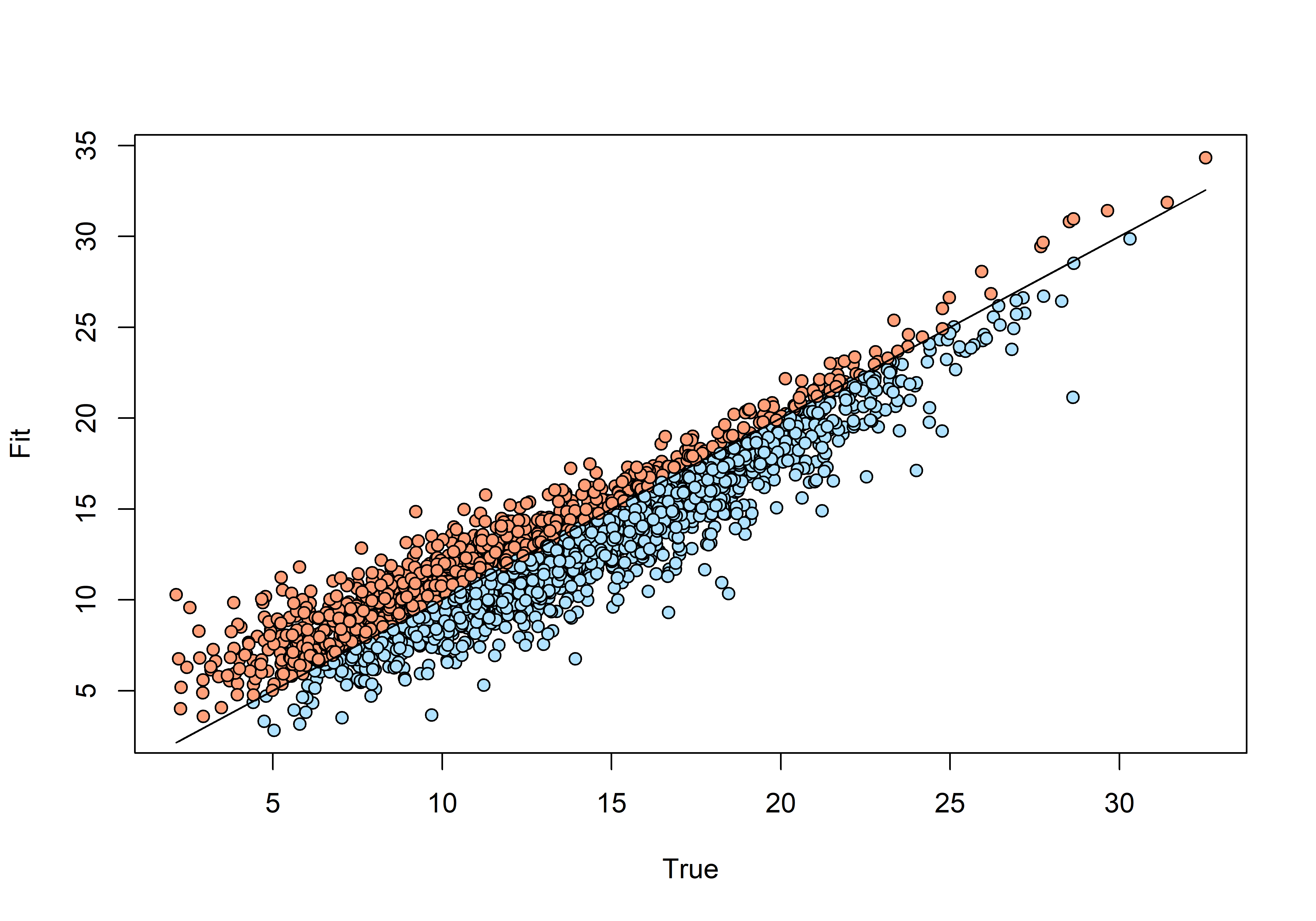
#### fit plotppc.df<-data.frame(fit =ppc.out.sp$fit.y, fit.rep =ppc.out.sp$fit.y.rep, color ='lightskyblue1')ppc.df$color[ppc.df$fit.rep.1>ppc.df$fit.1]<-'lightsalmon'plot(ppc.df$fit.1, ppc.df$fit.rep.1, bg =ppc.df$color, pch =21, ylab ='Fit', xlab ='True')lines(ppc.df$fit.1, ppc.df$fit.1, col ='black')
The most symmetrical, better fit!
Model comparison
Code
# 4. Model comparison -----------------------------------------------------# Compute Widely Applicable Information Criterion (WAIC)# Lower values indicate better model fit. waicOcc(out.null)
# Here we summarize the spatial factor loadings# summary(out.sp$lambda.samples)# Resultados --------------------------------------------------------------# Extraemos lo tabla de valores estimadosmodresult<-cbind(as.data.frame(waicOcc(out.null)),as.data.frame(waicOcc(out.sp)),as.data.frame(waicOcc(out.lfMs)),as.data.frame(waicOcc(out.sp.cat))#as.data.frame(waicOcc(out.sp.gaus)))# View(modresult)modresult_sorted<-as.data.frame(t(modresult))|>arrange(WAIC)# sort byDT::datatable(modresult_sorted)
Important
Lower values in WAIC indicate better model fit.
WAIC is the Widely Applicable Information Criterion (Watanabe 2010).
Posterior Summary
Code
# 5. Posterior summaries --------------------------------------------------# Concise summary of main parameter estimatessummary(out.sp, level ='community')
Bayesian p-values can be inspected to check for lack of fit (overall or by species). Lack of fit at significance level = 0.05 is indicated by Bayesian p-values below 0.025 or greater than 0.975. The overall Bayesian p-value (Bpvalue) indicates no problems with lack of fit. Likewise, species-level Bayesian p-values (Bpvalue_species) indicate no lack of fit for any species.
Gelman and Rubin’s convergence diagnostic: Approximate convergence is diagnosed when the upper limit is close to 1.
Convergence is diagnosed when the chains have ‘forgotten’ their initial values, and the output from all chains is indistinguishable. The gelman.diag diagnostic is applied to a single variable from the chain. It is based a comparison of within-chain and between-chain variances, and is similar to a classical analysis of variance.
Values substantially above 1 indicate lack of convergence.
Model Diagnostics
Code
#| eval: true#| echo: true#| code-fold: true#| warning: false#| message: false# Extract posterior draws for later useposterior1<-as.array(out.sp)# Trace plots to check chain mixing. Extract posterior samples and bind in a single matrix.POSTERIOR.MATRIX<-cbind(out.sp$alpha.comm.samples, out.sp$beta.comm.samples, out.sp$alpha.samples, out.sp$beta.samples)# Matrix output is all chains combined, split into 3 chains.CHAIN.1<-as.mcmc(POSTERIOR.MATRIX[1:1000,])CHAIN.2<-as.mcmc(POSTERIOR.MATRIX[1001:2000,])CHAIN.3<-as.mcmc(POSTERIOR.MATRIX[2001:3000,])# CHAIN.4 <- as.mcmc(POSTERIOR.MATRIX[8001:10000,])# Bind four chains as coda mcmc.list object.POSTERIOR.CHAINS<-mcmc.list(CHAIN.1, CHAIN.2, CHAIN.3)#, CHAIN.4)# Create an empty folder.# dir.create ("Beetle_plots")# Plot chain mixing of each parameter to a multi-panel plot and save to the new folder. ART 5 mins########################################## SAVE Diagnostics at PDF# MCMCtrace(POSTERIOR.CHAINS, params = "all", Rhat = TRUE, n.eff = TRUE)#, pdf = TRUE, filename = "Beetle_240909_traceplots.pdf", wd = "Beetle_plots")#mcmc_trace(fit.commu, parms = c("beta.ranef.cont.border_dist.mean"))#posterior2 <- extract(fit.commu, inc_warmup = TRUE, permuted = FALSE)#color_scheme_set("mix-blue-pink")#p <- mcmc_trace(posterior1, pars = c("mu", "tau"), n_warmup = 300,# facet_args = list(nrow = 2, labeller = label_parsed))#p + facet_text(size = 15)#outMCMC <- fit.commu #Convert output to MCMC object#diagnostics chains # all as pdf# MCMCtrace(outMCMC)# MCMCtrace(outMCMC, params = c("alpha0"), type = 'trace', Rhat = TRUE, n.eff = TRUE)# MCMCtrace(outMCMC, params = c("beta0"), type = 'trace', Rhat = TRUE, n.eff = TRUE)# MCMCtrace(outMCMC, params = c("beta.ranef.cont.border_dist"), type = 'trace', Rhat = TRUE, n.eff = TRUE)# MCMCtrace(out.sp, params = c("beta.ranef.cont.border_dist.mean"), type = 'trace', pdf = F, Rhat = TRUE, n.eff = TRUE)# MCMCtrace(outMCMC, params = c("beta.ranef.cont.elev"), type = 'trace', Rhat = TRUE, n.eff = TRUE)# MCMCtrace(outMCMC, params = c("beta.ranef.cont.elev.mean"), type = 'trace', pdf = F, Rhat = TRUE, n.eff = TRUE)### density# MCMCtrace(outMCMC, params = c("Nspecies"), ISB = FALSE, pdf = F, exact = TRUE, post_zm = TRUE, type = 'density', Rhat = TRUE, n.eff = TRUE, ind = TRUE)### density# MCMCtrace(outMCMC, params = c("beta.ranef.cont.elev.mean"), ISB = FALSE, pdf = F, exact = TRUE, post_zm = TRUE, type = 'density', Rhat = TRUE, n.eff = TRUE, ind = TRUE)### density#MCMCtrace(outMCMC, params = c("beta.ranef.cont.border_dist.mean"), ISB = FALSE, pdf = F, exact = TRUE, post_zm = TRUE, type = 'density', Rhat = TRUE, n.eff = TRUE, ind = TRUE)#coda::gelman.diag(outMCMC, multivariate = FALSE, transform=FALSE)# coda::gelman.plot(outMCMC, multivariate = FALSE)# # mcmc_intervals(outMCMC, pars = c("Nspecies_in_AP[1]",# "Nspecies_in_AP[2]"),# point_est = "mean",# prob = 0.75, prob_outer = 0.95) +# ggtitle("Number of species") + # scale_y_discrete(labels = c("Nspecies_in_AP[1]"=levels(sitecovs$in_AP)[1],# "Nspecies_in_AP[2]"=levels(sitecovs$in_AP)[2]))# # #Continuous# p <- mcmc_intervals(outMCMC, # pars = c("beta.ranef.cont.border_dist.mean",# #"beta.ranef.cont.elev.mean",# "beta.ranef.categ.in_AP.mean[2]"))# # # relabel parameters# p + scale_y_discrete(# labels = c("beta.ranef.cont.border_dist.mean"="Dist_border",# #"beta.ranef.cont.elev.mean"="Elevation",# "beta.ranef.categ.in_AP.mean[2]"="in_AP")# ) +# ggtitle("Treatment effect on all species")#
Posterior Summary (effect)
Community effects
Code
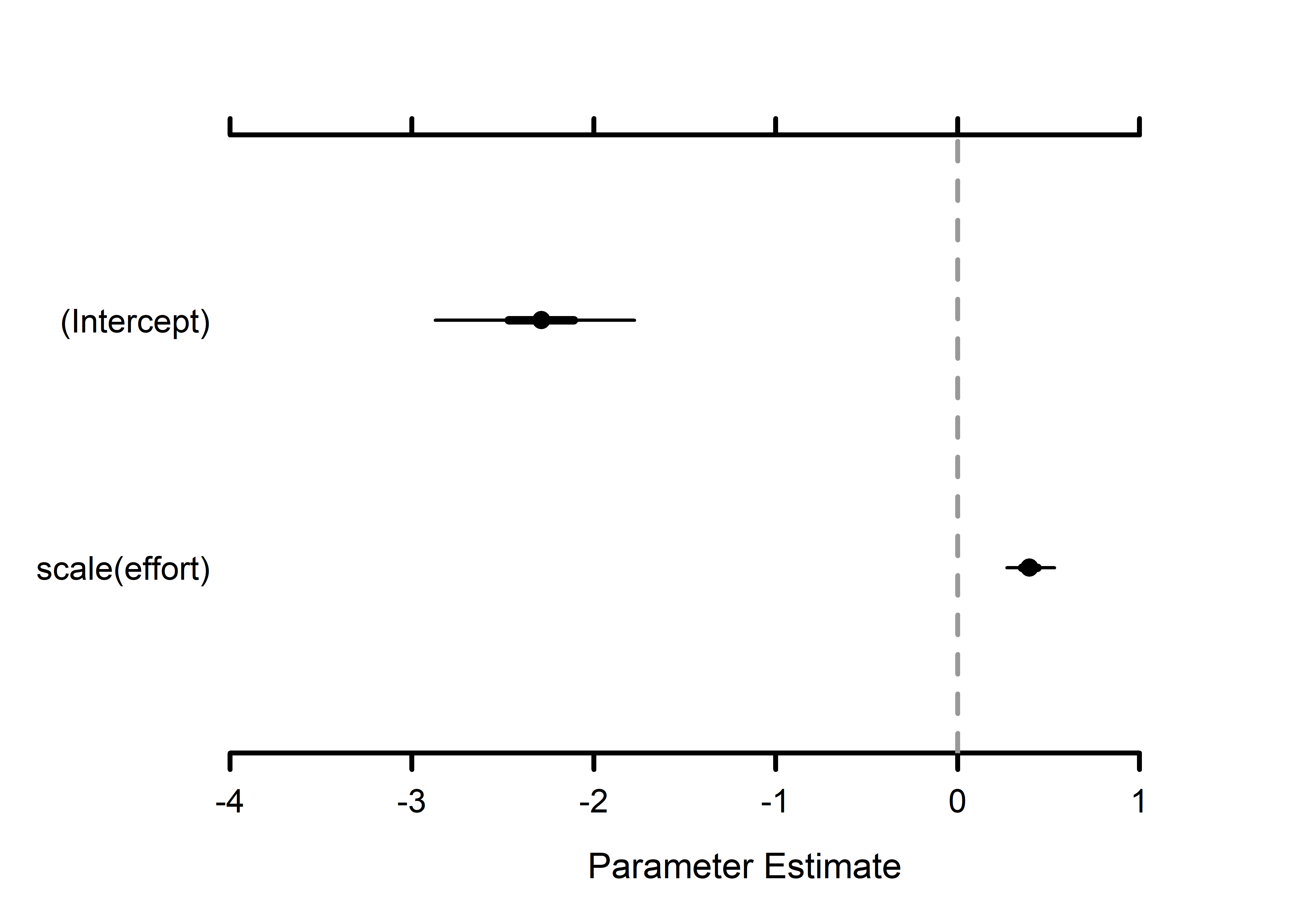
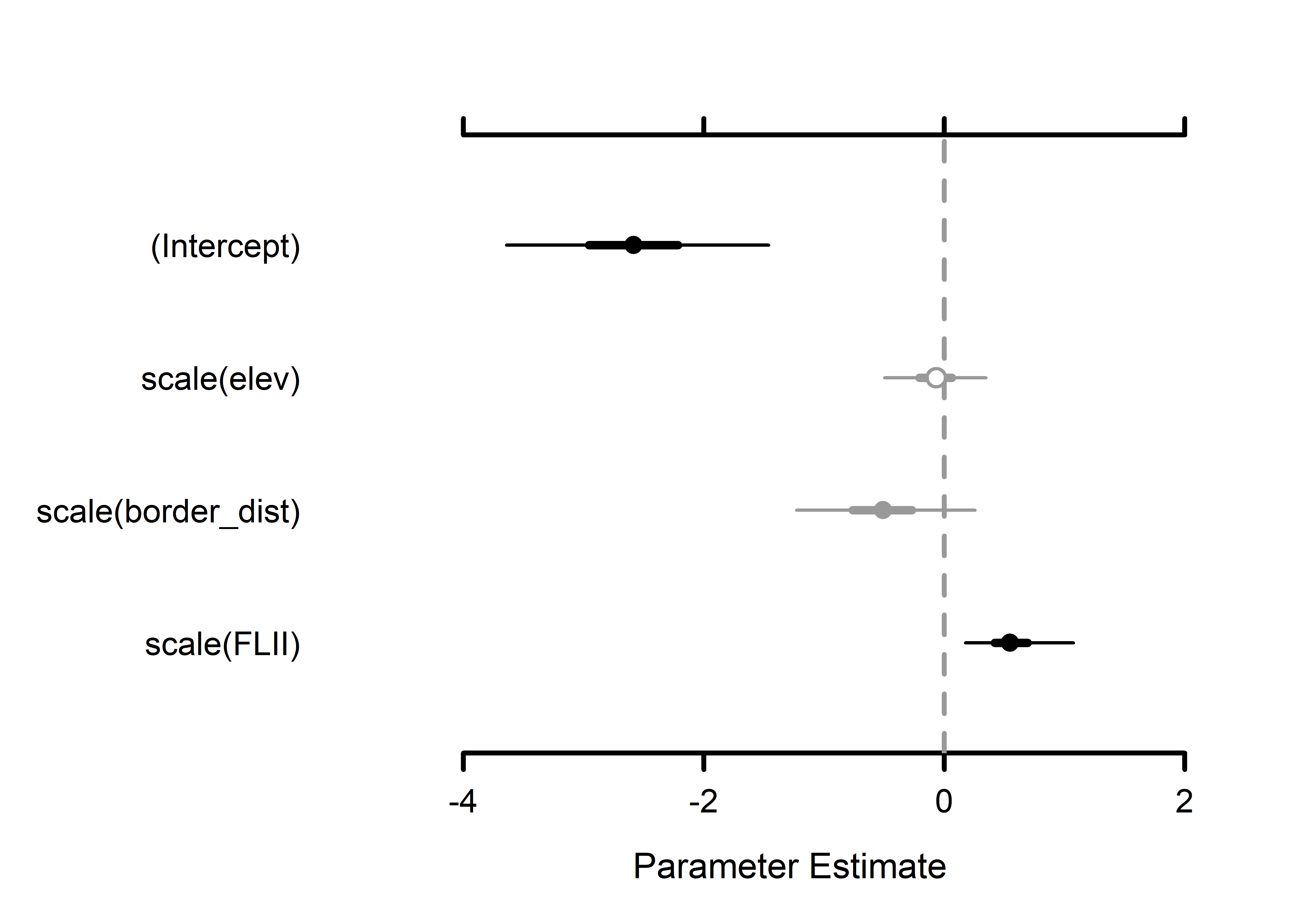
# Create simple plot summaries using MCMCvis package.# Detection covariate effects --------- MCMCplot(out.sp$alpha.comm.samples, ref_ovl =TRUE, ci =c(50, 95))# Occupancy community-level effects MCMCplot(out.sp$beta.comm.samples, ref_ovl =TRUE, ci =c(50, 95))
(a) Detection
(b) Occupancy
Figure 1: Community effects
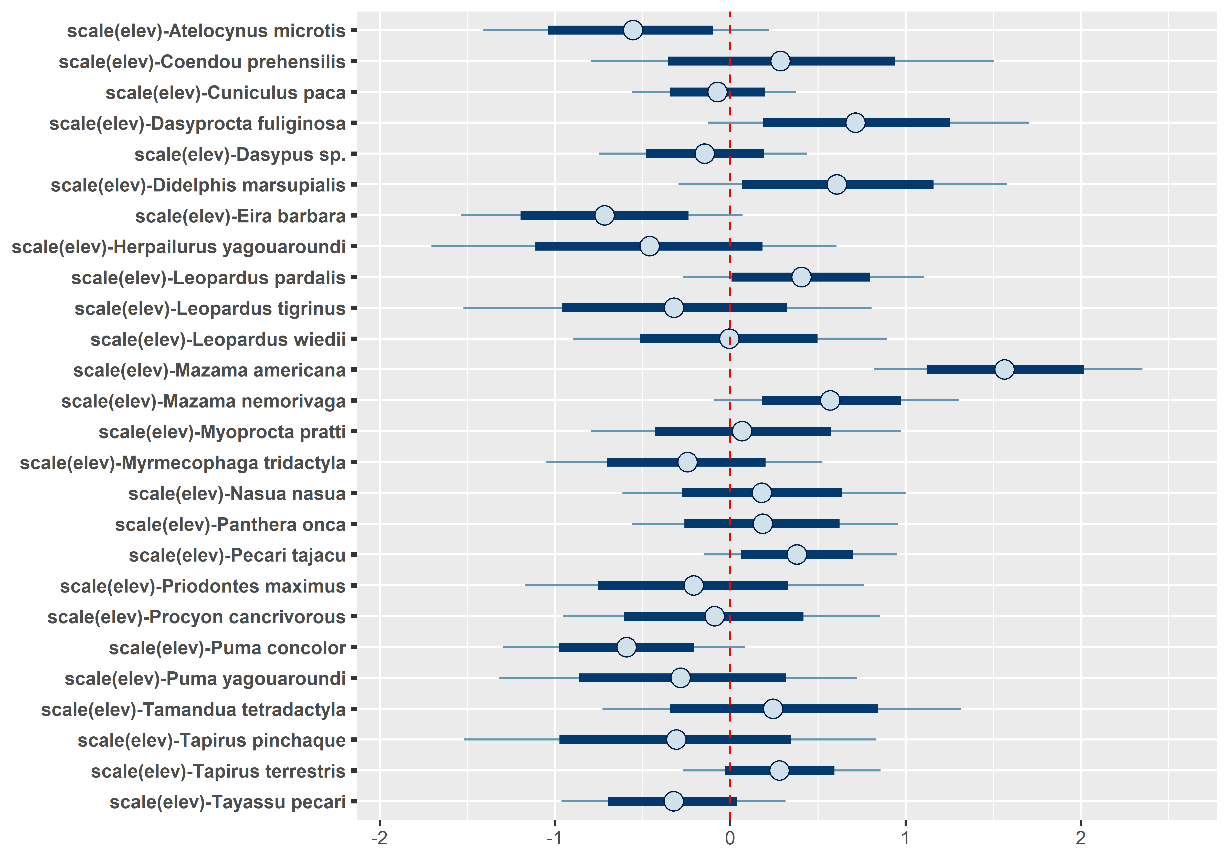
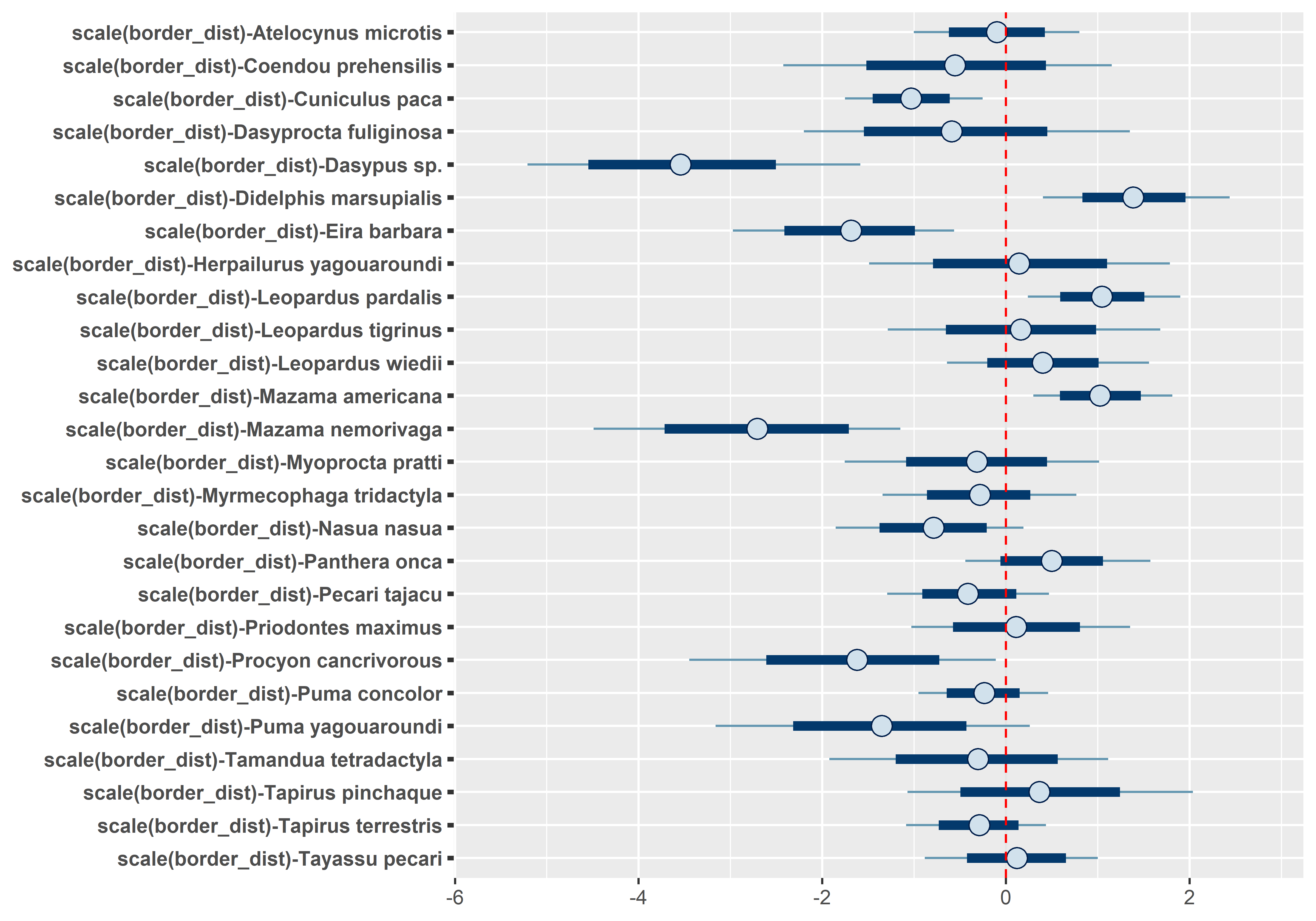
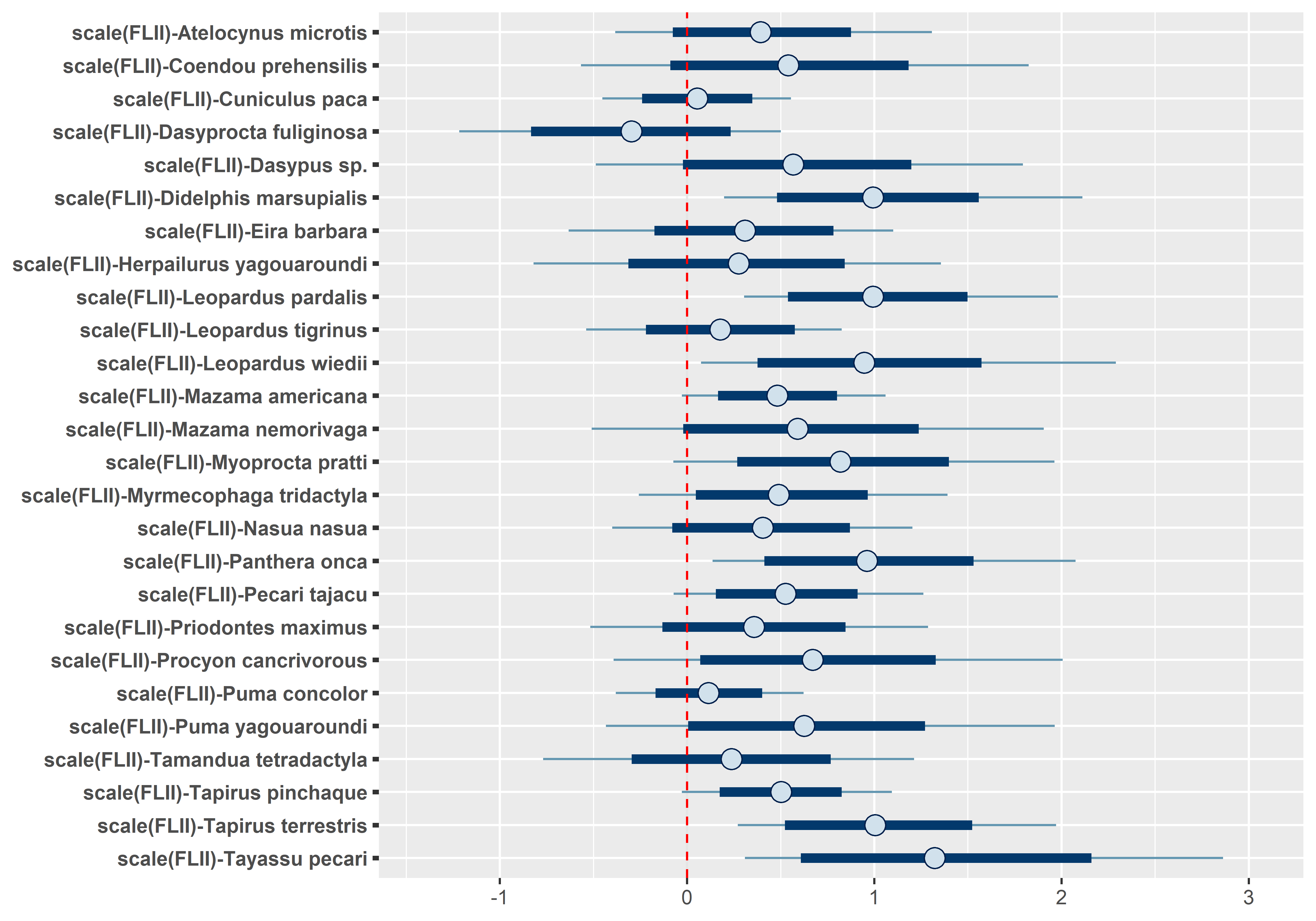
Species effects
Code
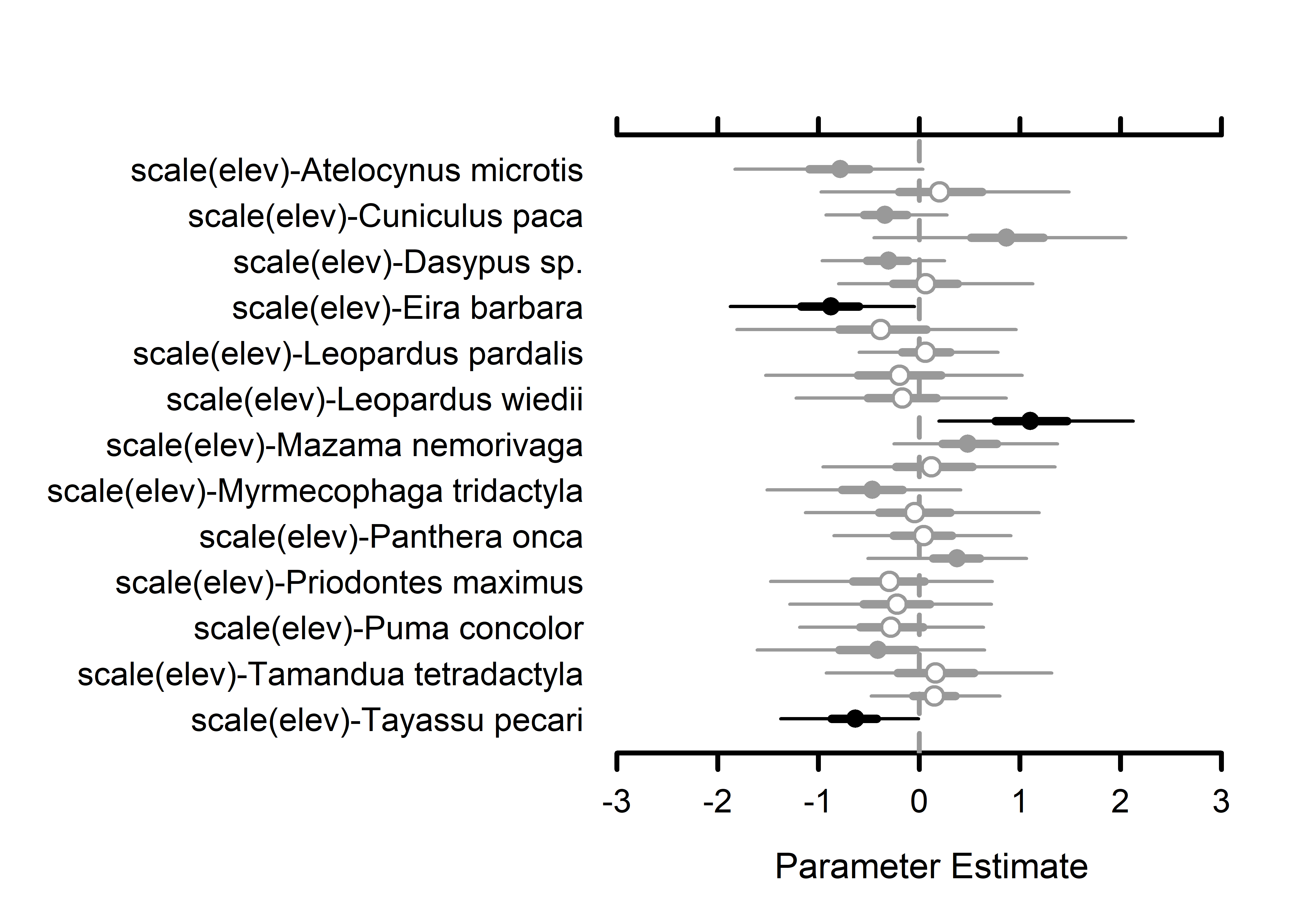
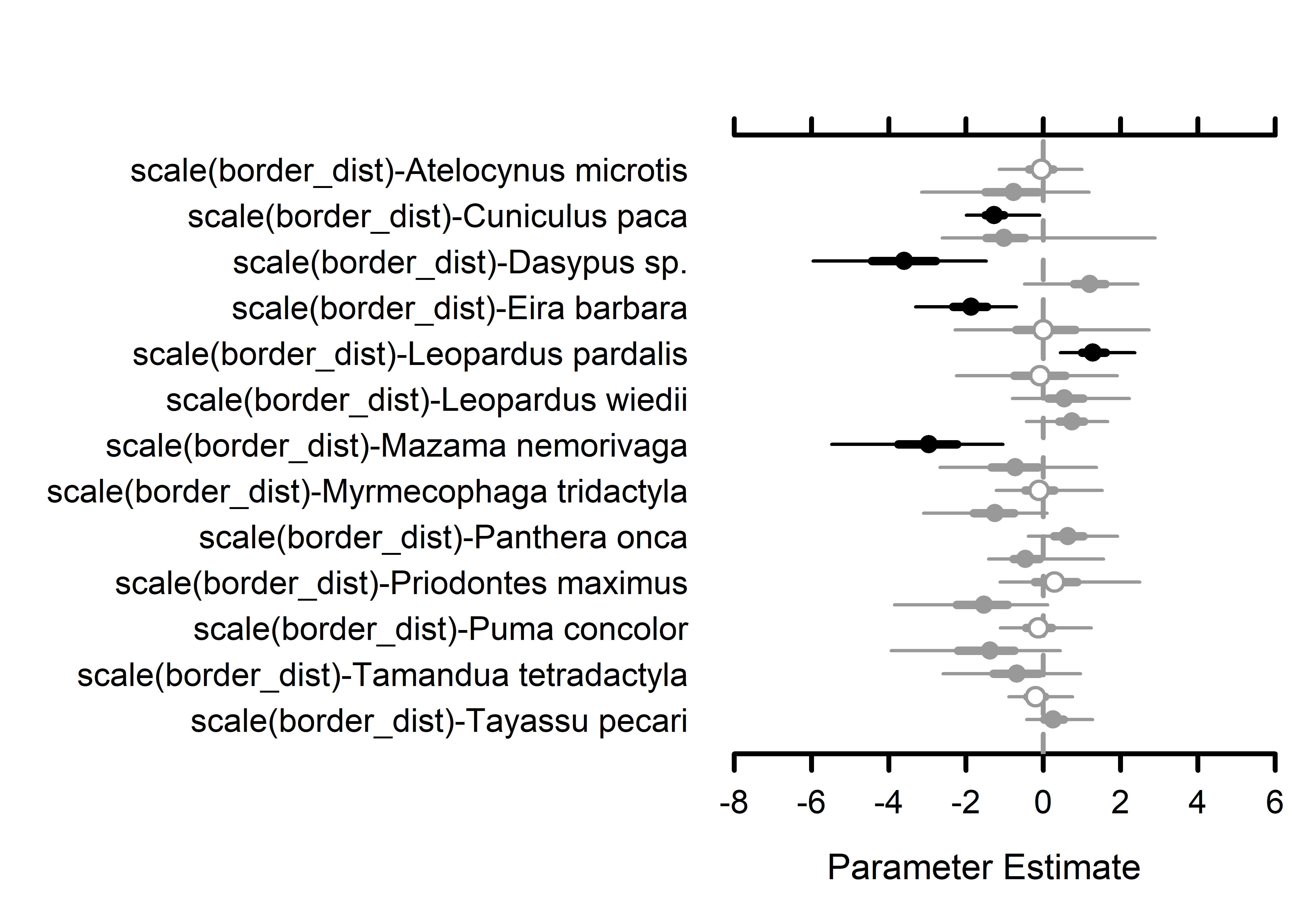
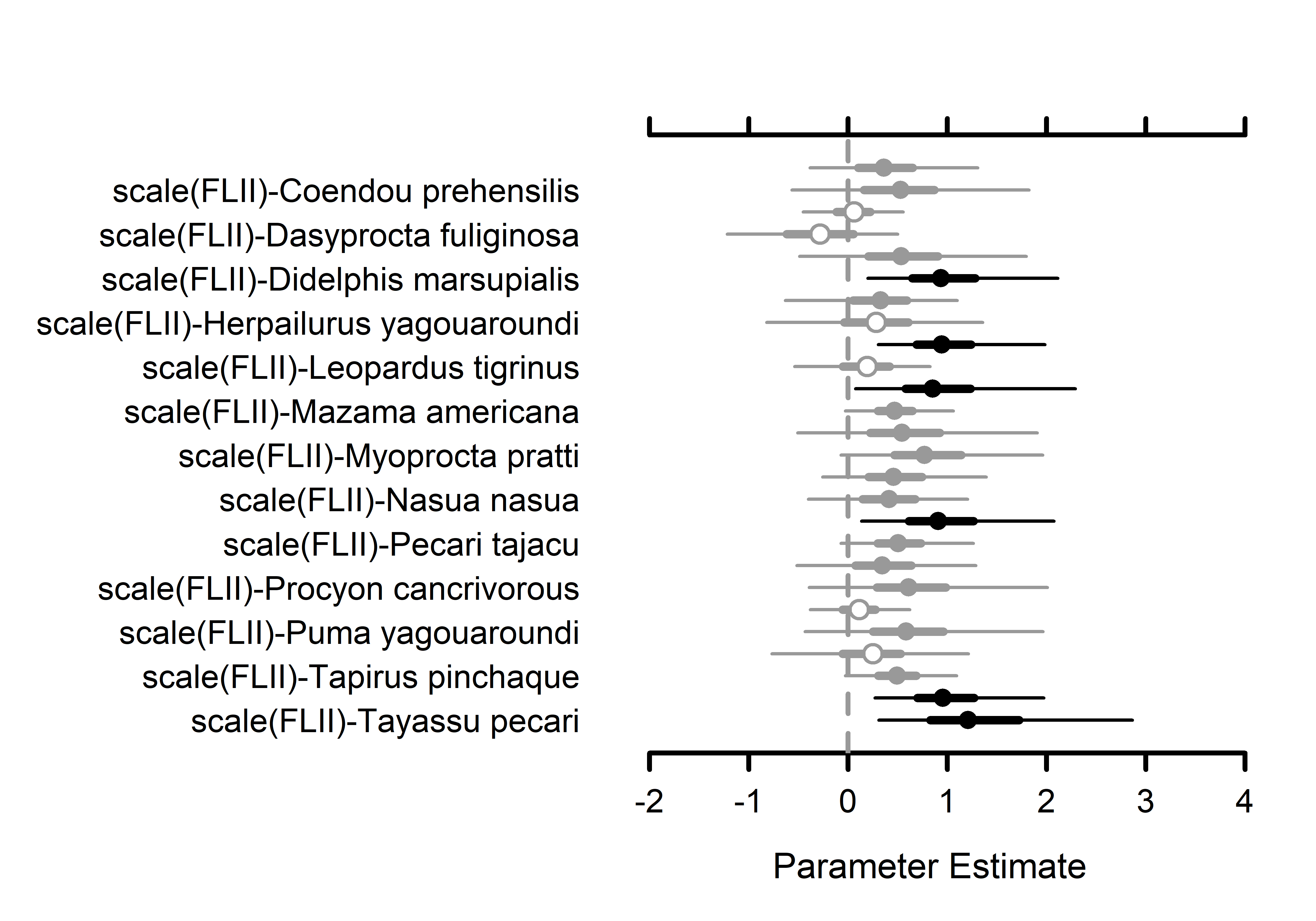
# Occupancy species-level effects MCMCplot(out.sp$beta.samples[,27:52], ref_ovl =TRUE, ci =c(50, 95))# Occupancy species-level effects MCMCplot(out.sp$beta.samples[,53:78], ref_ovl =TRUE, ci =c(50, 95))# Occupancy species-level effects MCMCplot(out.sp$beta.samples[,79:104], ref_ovl =TRUE, ci =c(50, 95))
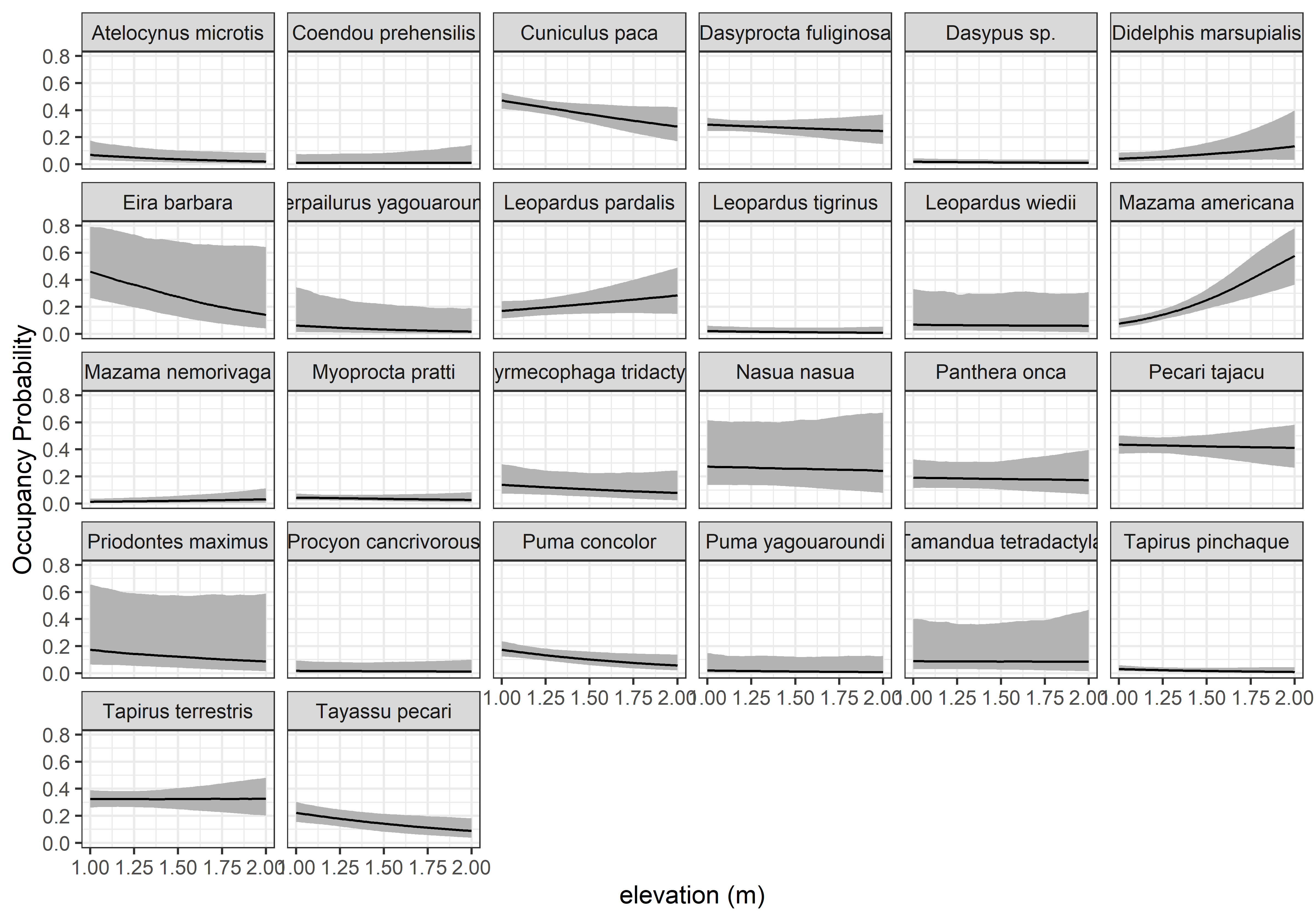
# 6. Prediction -----------------------------------------------------------# Predict occupancy along a gradient of elev # Create a set of values across the range of observed elev valueselev.pred.vals<-seq(min(data_list$occ.covs$elev), max(data_list$occ.covs$elev), length.out =100)# Scale predicted values by mean and standard deviation used to fit the modelelev.pred.vals.scale<-(elev.pred.vals-mean(data_list$occ.covs$elev))/sd(data_list$occ.covs$elev)# Create a set of values across the range of observed elev valuesborder_dist.pred.vals<-seq(min(data_list$occ.covs$border_dist), max(data_list$occ.covs$border_dist), length.out =100)# Scale predicted values by mean and standard deviation used to fit the modelborder_dist.pred.vals.scale<-(border_dist.pred.vals-mean(data_list$occ.covs$border_dist))/sd(data_list$occ.covs$border_dist)# Create a set of values across the range of observed FLII valuesFLII.pred.vals<-seq(min(data_list$occ.covs$FLII), max(data_list$occ.covs$FLII), length.out =100)# Scale predicted values by mean and standard deviation used to fit the modelFLII.pred.vals.scale<-(FLII.pred.vals-mean(data_list$occ.covs$FLII))/sd(data_list$occ.covs$FLII)# Predict occupancy across elev values at mean values of all other variablespred.df1<-as.matrix(data.frame(intercept =1, elev =elev.pred.vals.scale, border_dist =0, FLII=0))#, catchment = 0, density = 0, # slope = 0))# Predict occupancy across elev values at mean values of all other variablespred.df2<-as.matrix(data.frame(intercept =1, elev =0, border_dist =border_dist.pred.vals.scale, FLII=0))#, catchment = 0, density = 0, # slope = 0))# Predict occupancy across elev values at mean values of all other variablespred.df3<-as.matrix(data.frame(intercept =1, elev =0, border_dist =0, FLII=FLII.pred.vals.scale))#, catchment = 0, density = 0, # slope = 0))out.pred1<-predict(out.null, pred.df1)# using non spatialstr(out.pred1)
List of 3
$ psi.0.samples: num [1:1500, 1:26, 1:100] 0.0331 0.0329 0.052 0.0469 0.0381 ...
$ z.0.samples : int [1:1500, 1:26, 1:100] 0 0 0 0 0 0 0 0 0 0 ...
$ call : language predict.msPGOcc(object = out.null, X.0 = pred.df1)
- attr(*, "class")= chr "predict.msPGOcc"
Code
psi.0.quants<-apply(out.pred1$psi.0.samples, c(2, 3), quantile, prob =c(0.025, 0.5, 0.975))sp.codes<-attr(data_list$y, "dimnames")[[1]]psi.plot.dat<-data.frame(psi.med =c(t(psi.0.quants[2, , ])), psi.low =c(t(psi.0.quants[1, , ])), psi.high =c(t(psi.0.quants[3, , ])), elev =elev.pred.vals, sp.codes =rep(sp.codes, each =length(elev.pred.vals)))ggplot(psi.plot.dat, aes(x =elev, y =psi.med))+geom_ribbon(aes(ymin =psi.low, ymax =psi.high), fill ='grey70')+geom_line()+facet_wrap(vars(sp.codes))+theme_bw()+labs(x ='elevation (m)', y ='Occupancy Probability')
Code
out.pred2<-predict(out.null, pred.df2)# using non spatialstr(out.pred2)
List of 3
$ psi.0.samples: num [1:1500, 1:26, 1:100] 0.0271 0.0287 0.1033 0.0633 0.0257 ...
$ z.0.samples : int [1:1500, 1:26, 1:100] 0 0 0 0 0 0 0 0 0 0 ...
$ call : language predict.msPGOcc(object = out.null, X.0 = pred.df2)
- attr(*, "class")= chr "predict.msPGOcc"
Code
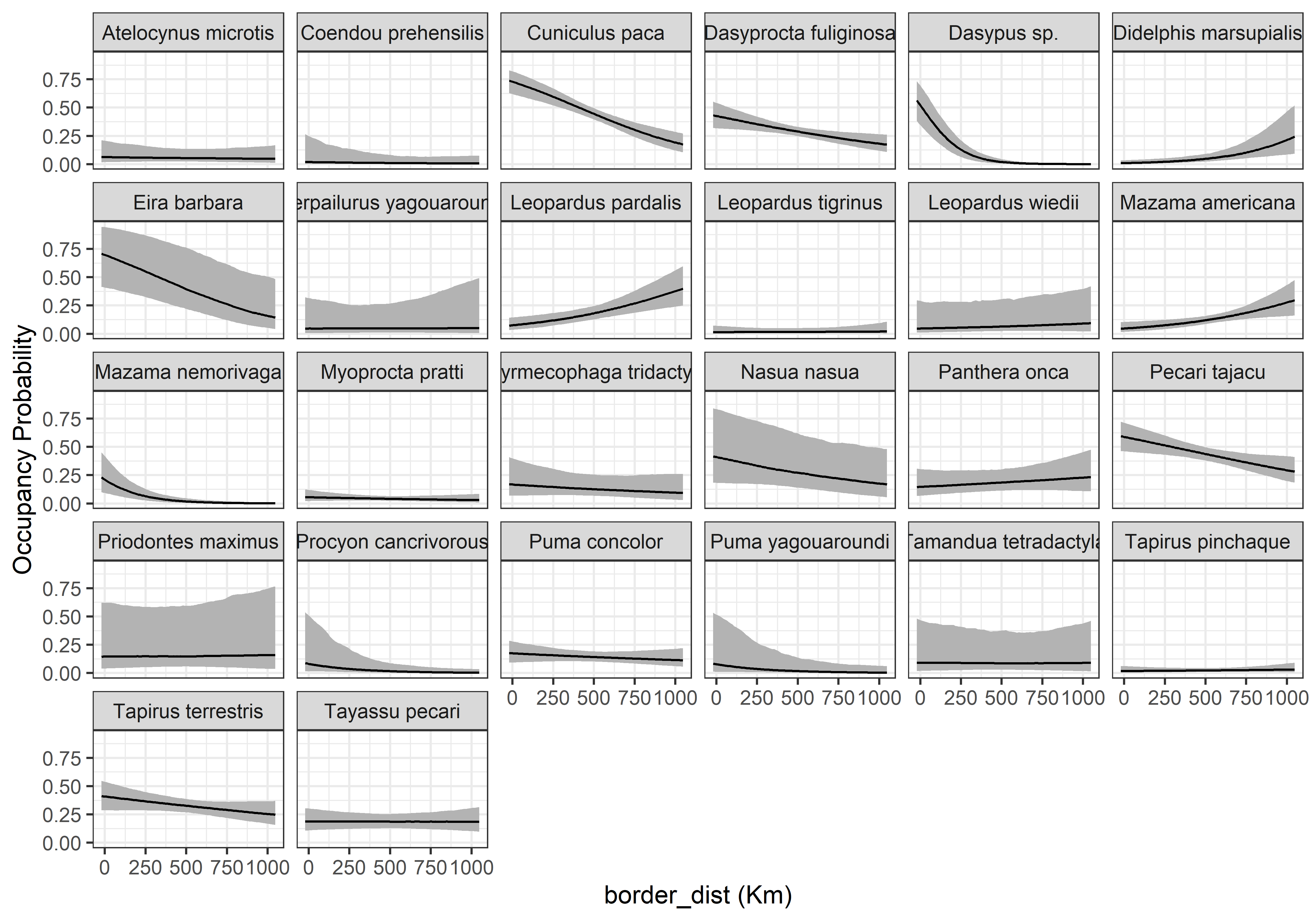
psi.0.quants<-apply(out.pred2$psi.0.samples, c(2, 3), quantile, prob =c(0.025, 0.5, 0.975))sp.codes<-attr(data_list$y, "dimnames")[[1]]psi.plot.dat<-data.frame(psi.med =c(t(psi.0.quants[2, , ])), psi.low =c(t(psi.0.quants[1, , ])), psi.high =c(t(psi.0.quants[3, , ])), border_dist =border_dist.pred.vals, sp.codes =rep(sp.codes, each =length(border_dist.pred.vals)))ggplot(psi.plot.dat, aes(x =border_dist/1000, y =psi.med))+geom_ribbon(aes(ymin =psi.low, ymax =psi.high), fill ='grey70')+geom_line()+facet_wrap(vars(sp.codes))+theme_bw()+labs(x ='border_dist (Km)', y ='Occupancy Probability')
Code
out.pred3<-predict(out.null, pred.df3)# using non spatialstr(out.pred3)
List of 3
$ psi.0.samples: num [1:1500, 1:26, 1:100] 0.00265 0.00346 0.00313 0.01032 0.00231 ...
$ z.0.samples : int [1:1500, 1:26, 1:100] 0 0 0 0 0 0 0 0 0 0 ...
$ call : language predict.msPGOcc(object = out.null, X.0 = pred.df3)
- attr(*, "class")= chr "predict.msPGOcc"
Code
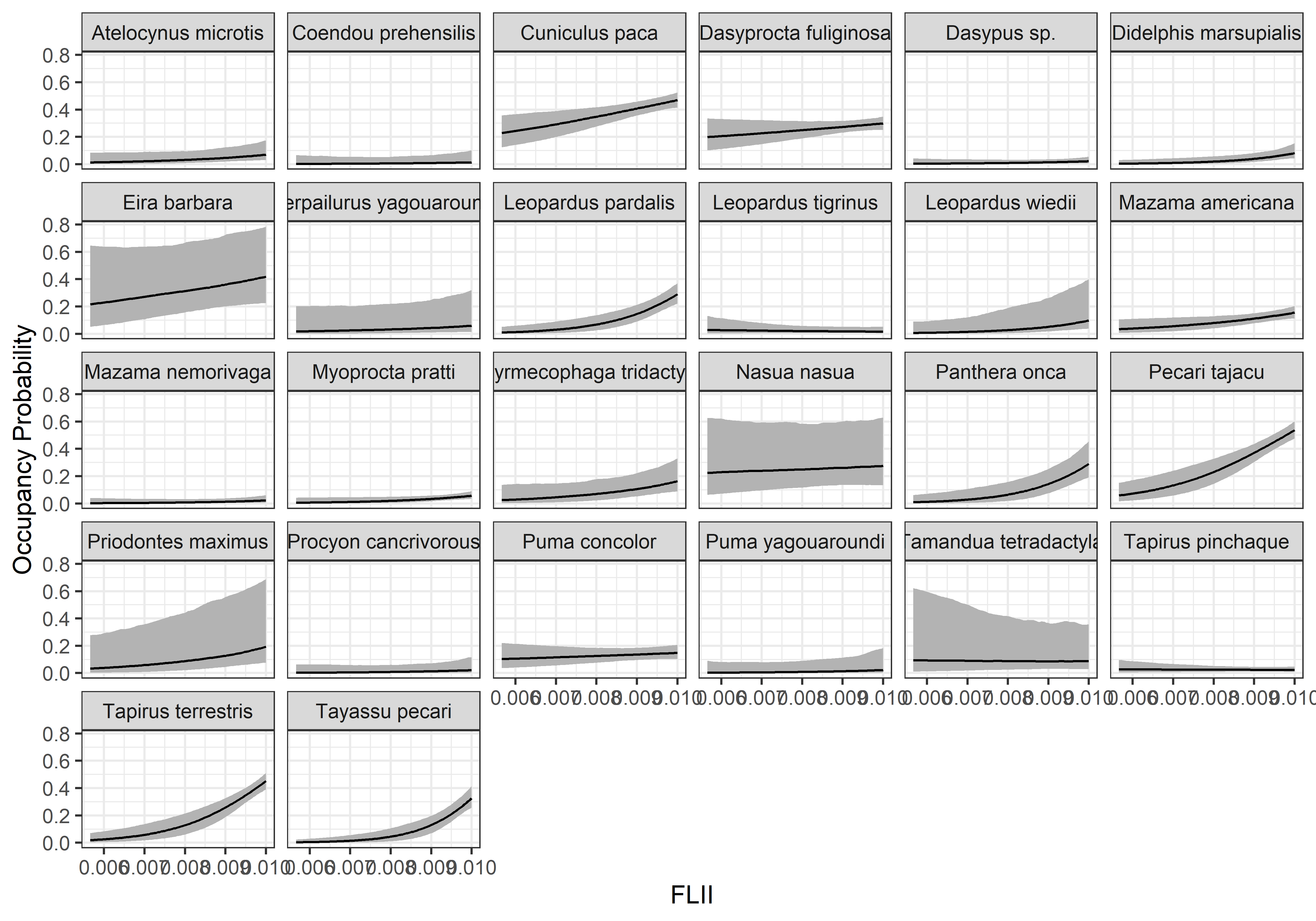
psi.0.quants<-apply(out.pred3$psi.0.samples, c(2, 3), quantile, prob =c(0.025, 0.5, 0.975))sp.codes<-attr(data_list$y, "dimnames")[[1]]psi.plot.dat<-data.frame(psi.med =c(t(psi.0.quants[2, , ])), psi.low =c(t(psi.0.quants[1, , ])), psi.high =c(t(psi.0.quants[3, , ])), FLII =FLII.pred.vals, sp.codes =rep(sp.codes, each =length(FLII.pred.vals)))ggplot(psi.plot.dat, aes(x =FLII/1000, y =psi.med))+geom_ribbon(aes(ymin =psi.low, ymax =psi.high), fill ='grey70')+geom_line()+facet_wrap(vars(sp.codes))+theme_bw()+labs(x ='FLII', y ='Occupancy Probability')
Spatial Prediction in elevation_EC
Code
#aggregate resolution to (factor = 3)#transform coord data to UTMelevation_UTM<-project(elevation_EC, "EPSG:10603")elevation_17.aggregate<-aggregate(elevation_UTM, fact=10)res(elevation_17.aggregate)
[1] 5984.313 5984.313
Code
# Convert the SpatRaster to a data frame with coordinatesdf_coords<-as.data.frame(elevation_17.aggregate, xy =TRUE)names(df_coords)<-c("X","Y","elev")elev.pred<-(df_coords$elev-mean(data_list$occ.covs$elev))/sd(data_list$occ.covs$elev)############### Predict new data ############### # we predict at one covariate varing and others at mean value = 0# intercept = 1, elev = 0, border_dist = 0, FLII= 0# in that order################ ################ ################ predict_data<-cbind(1, elev.pred, 0, 0)colnames(predict_data)<-c("intercept","elev","border_dist","FLII")# X.0 <- cbind(1, 1, elev.pred)#, elev.pred^2)# coords.0 <- as.matrix(hbefElev[, c('Easting', 'Northing')])out.sp.ms.pred<-predict(out.sp, X.0=predict_data, df_coords[,1:2], threads=4)#Warning :'threads' is not an argument
Warning in predict.sfMsPGOcc(out.sp, X.0 = predict_data, df_coords[, 1:2], :
'threads' is not an argument
----------------------------------------
Prediction description
----------------------------------------
Spatial Factor NNGP Multispecies Occupancy model with Polya-Gamma latent
variable fit with 514 observations.
Number of covariates 4 (including intercept if specified).
Using the exponential spatial correlation model.
Using 15 nearest neighbors.
Using 5 latent spatial factors.
Number of MCMC samples 3000.
Predicting at 2618 non-sampled locations.
Source compiled with OpenMP support and model fit using 1 threads.
-------------------------------------------------
Predicting
-------------------------------------------------
Location: 100 of 2618, 3.82%
Location: 200 of 2618, 7.64%
Location: 300 of 2618, 11.46%
Location: 400 of 2618, 15.28%
Location: 500 of 2618, 19.10%
Location: 600 of 2618, 22.92%
Location: 700 of 2618, 26.74%
Location: 800 of 2618, 30.56%
Location: 900 of 2618, 34.38%
Location: 1000 of 2618, 38.20%
Location: 1100 of 2618, 42.02%
Location: 1200 of 2618, 45.84%
Location: 1300 of 2618, 49.66%
Location: 1400 of 2618, 53.48%
Location: 1500 of 2618, 57.30%
Location: 1600 of 2618, 61.12%
Location: 1700 of 2618, 64.94%
Location: 1800 of 2618, 68.75%
Location: 1900 of 2618, 72.57%
Location: 2000 of 2618, 76.39%
Location: 2100 of 2618, 80.21%
Location: 2200 of 2618, 84.03%
Location: 2300 of 2618, 87.85%
Location: 2400 of 2618, 91.67%
Location: 2500 of 2618, 95.49%
Location: 2600 of 2618, 99.31%
Location: 2618 of 2618, 100.00%
Generating latent occupancy state
Code
# extract the array of interest= occupancypredicted_array<-out.sp.ms.pred$psi.0.samplesdim(predicted_array)
[1] 3000 26 2618
Code
# df_plot <- NA # empty columnpredicted_raster_list<-list()# rast(nrows = 52, ncols = 103,#ext(elevation_17.aggregate), # crs = "EPSG:32717")#################################################### simpler way to make mean in the array by species# array order: itera=3000, sp=22, pixels=5202# we wan to keep index 2 and 3library(plyr)
You have loaded plyr after dplyr - this is likely to cause problems.
If you need functions from both plyr and dplyr, please load plyr first, then dplyr:
library(plyr); library(dplyr)
The following objects are masked from 'package:dplyr':
arrange, count, desc, failwith, id, mutate, rename, summarise,
summarize
The following object is masked from 'package:purrr':
compact
The following object is masked from 'package:maps':
ozone
Code
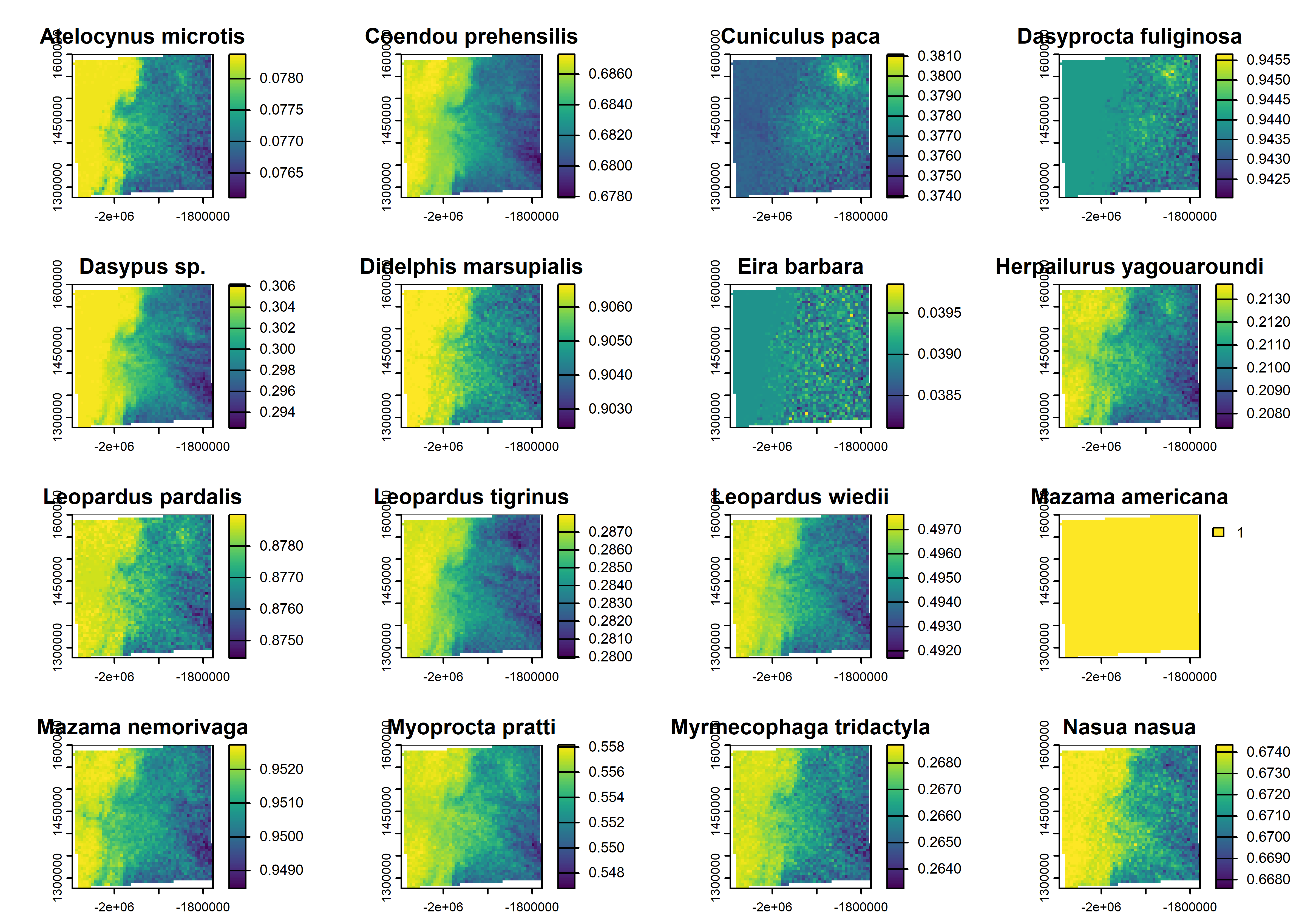
aresult=(plyr::aaply(predicted_array, # mean fo all iterationsc(2,3), mean))################################################## Loop to make rasters and put in a list# array order: itera=3000, sp=22, pixels=5202for(iin1:dim(predicted_array)[2]){# Convert array slice to data frame# df_plot[i] <- as.data.frame(predicted_array[1, i, ]) # sp_i# df_plot[i] <- as.vector(aresult[i,]) # Extract sp# Producing an SDM for all (posterior mean)plot.dat<-data.frame(x =df_coords$X, y =df_coords$Y, psi.sp =as.vector(aresult[i,]))pred_rast<-rast(plot.dat, type ="xyz", crs ="EPSG:10603")# Replace EPSG:4326 with your CRSpredicted_raster_list[[i]]<-pred_rast}# Convert the list to a SpatRaster stackpredictad_raster_stack<-rast(predicted_raster_list)# put species namesnames(predictad_raster_stack)<-selected.spplot(predictad_raster_stack)
Code
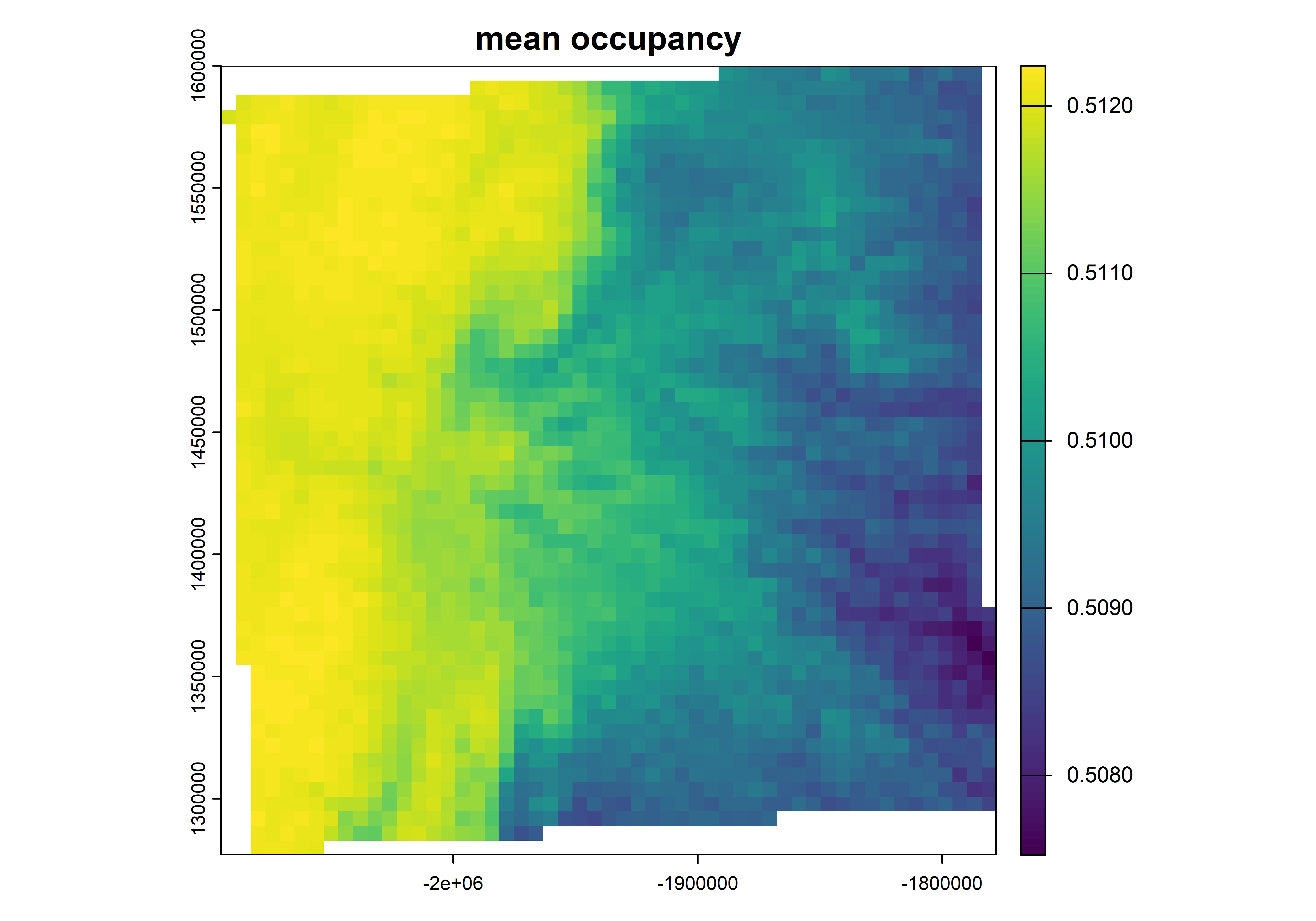
# get the meanpredicted_mean<-mean(predictad_raster_stack)plot(predicted_mean, main="mean occupancy")
Appelhans, Tim, Florian Detsch, Christoph Reudenbach, and Stefan Woellauer. 2025. mapview: Interactive Viewing of Spatial Data in r. https://CRAN.R-project.org/package=mapview.
Becker, Richard A., Allan R. Wilks, Ray Brownrigg, Thomas P. Minka, and Alex Deckmyn. 2025. maps: Draw Geographical Maps. https://CRAN.R-project.org/package=maps.
Doser, Jeffrey W., Andrew O. Finley, and Sudipto Banerjee. 2023. “Joint Species Distribution Models with Imperfect Detection for High-Dimensional Spatial Data.”Ecology, e4137. https://doi.org/10.1002/ecy.4137.
Doser, Jeffrey W., Andrew O. Finley, Marc Kéry, and Elise F. Zipkin. 2022. “spOccupancy: An r Package for Single-Species, Multi-Species, and Integrated Spatial Occupancy Models.”Methods in Ecology and Evolution 13: 1670–78. https://doi.org/10.1111/2041-210X.13897.
Doser, Jeffrey W., Andrew O. Finley, Sarah P. Saunders, Marc Kéry, Aaron S. Weed, and Elise F. Zipkin. 2024. “Modeling Complex Species-Environment Relationships Through Spatially-Varying Coefficient Occupancy Models.”Journal of Agricultural, Biological, and Environmental Statistics. https://doi.org/10.1007/s13253-023-00595-6.
Gabry, Jonah, Daniel Simpson, Aki Vehtari, Michael Betancourt, and Andrew Gelman. 2019. “Visualization in Bayesian Workflow.”J. R. Stat. Soc. A 182: 389–402. https://doi.org/10.1111/rssa.12378.
Hollister, Jeffrey, Tarak Shah, Jakub Nowosad, Alec L. Robitaille, Marcus W. Beck, and Mike Johnson. 2023. elevatr: Access Elevation Data from Various APIs. https://doi.org/10.5281/zenodo.8335450.
Izrailev, Sergei. 2024. tictoc: Functions for Timing r Scripts, as Well as Implementations of “Stack” and “StackList” Structures. https://CRAN.R-project.org/package=tictoc.
Niedballa, Jürgen, Rahel Sollmann, Alexandre Courtiol, and Andreas Wilting. 2016. “camtrapR: An r Package for Efficient Camera Trap Data Management.”Methods in Ecology and Evolution 7 (12): 1457–62. https://doi.org/10.1111/2041-210X.12600.
Pebesma, Edzer. 2018. “Simple Features for R: Standardized Support for Spatial Vector Data.”The R Journal 10 (1): 439–46. https://doi.org/10.32614/RJ-2018-009.
Plummer, Martyn, Nicky Best, Kate Cowles, and Karen Vines. 2006. “CODA: Convergence Diagnosis and Output Analysis for MCMC.”R News 6 (1): 7–11. https://journal.r-project.org/archive/.
R Core Team. 2024. R: A Language and Environment for Statistical Computing. Vienna, Austria: R Foundation for Statistical Computing. https://www.R-project.org/.
Wickham, Hadley. 2011. “The Split-Apply-Combine Strategy for Data Analysis.”Journal of Statistical Software 40 (1): 1–29. https://www.jstatsoft.org/v40/i01/.
Wickham, Hadley, Mara Averick, Jennifer Bryan, Winston Chang, Lucy D’Agostino McGowan, Romain François, Garrett Grolemund, et al. 2019. “Welcome to the tidyverse.”Journal of Open Source Software 4 (43): 1686. https://doi.org/10.21105/joss.01686.
Xie, Yihui, Joe Cheng, Xianying Tan, and Garrick Aden-Buie. 2025. DT: A Wrapper of the JavaScript Library “DataTables”. https://CRAN.R-project.org/package=DT.
Youngflesh, Casey. 2018. “MCMCvis: Tools to Visualize, Manipulate, and Summarize MCMC Output.”Journal of Open Source Software 3 (24): 640. https://doi.org/10.21105/joss.00640.
@online{forero2025,
author = {Forero, German and Wallace, Robert and Zapara-Rios, Galo and
Isasi-Catalá, Emiliana and J. Lizcano, Diego},
title = {Fitting a {Spatial} {Factor} {Multi-Species} {Occupancy}
{Model}},
date = {2025-08-16},
url = {https://dlizcano.github.io/Occu_APs_all/blog/2025-10-15-analysis/},
langid = {en}
}