Multispecies occupancy model

A new extension of camtrapR for community occupancy models

Multispecies occupancy models combines information from multiple species to estimate both individual and community-level responses to environmental variables
R
occupancy
JAGS
camtrapR
Author
Affiliation

Diego J. Lizcano

WildMon

Published

June 23, 2024

Using CamtrapR

CamtrapR is making very easy to make Multispecies occupancy models from camera trap data. Here one example.

Load packages

First we load some packages

Code

library(grateful) # Facilitate Citation of R Packages
library(patchwork) # The Composer of Plots
library(readxl) # Read Excel Files
library(sf) # Simple Features for R
library(mapview) # Interactive Viewing of Spatial Data in R
library(terra) # Spatial Data Analysis
library(elevatr) # Access Elevation Data from Various APIs

library(camtrapR) # Camera Trap Data Management and Preparation of Occupancy and Spatial Capture-Recapture Analyses 
library(rjags) # Bayesian Graphical Models using MCMC 
library(nimble) # MCMC, Particle Filtering, and Programmable Hierarchical Modeling 

library(bayesplot) # Plotting for Bayesian Models # Plotting for Bayesian Models 
library(SpadeR) # Species-Richness Prediction and Diversity Estimation with R 
library(tictoc) # Functions for Timing R Scripts, as Well as Implementations of "Stack" and "StackList" Structures 
library(beepr) # Easily Play Notification Sounds on any Platform 
library(snowfall) # Easier Cluster Computing (Based on 'snow')
library(bayesplot) # Plotting for Bayesian Models # Plotting for Bayesian Models 

library(kableExtra) # Construct Complex Table with 'kable' and Pipe Syntax
library(tidyverse) # Easily Install and Load the 'Tidyverse'

Load data

The data set is i a excel file so we use read_excel function to load it.

Code

datos <- read_excel("C:/CodigoR/CameraTrapCesar/data/CT_Cesar.xlsx")

Selecting Just CT_Becerril 2021

To this example I selected just one place one year, Becerril 2021. Sometimes we need to make unique codes per camera and cameraOperation table.

Code
# make a new column Station
# datos_PCF <- datos |> dplyr::filter(Proyecto=="CT_LaPaz_Manaure") |> unite ("Station", ProyectoEtapa:Salida:CT, sep = "-")

# fix dates
datos$Start <- as.Date(datos$Start, "%d/%m/%Y")
datos$End <- as.Date(datos$End, "%d/%m/%Y")
datos$eventDate <- as.Date(datos$eventDate, "%d/%m/%Y")
datos$eventDateTime <- ymd_hms(paste(datos$eventDate, " ",
                              datos$eventTime, ":00", sep=""))

# filter Becerril
datos_PCF <- datos |> dplyr::filter(ProyectoEtapa=="CT_Becerril") |> mutate (Station=IdGeo)

# filter 2021 and make uniques
CToperation  <- datos_PCF |> filter(Year==2021) |> group_by(Station) |> 
                           mutate(minStart=min(Start), maxEnd=max(End)) |> distinct(Longitude, Latitude, minStart, maxEnd, Year) |> ungroup()

Generating cameraOperation and making detection histories for all the species.

The package CamtrapR has the function ‘cameraOperation’ which makes a table of cameras (stations) and dates (setup, puck-up), this table is key to generate the detection histories using the function ‘detectionHistory’ in the next step.

Code
# Generamos la matríz de operación de las cámaras

camop <- cameraOperation(CTtable= CToperation, # Tabla de operación
                         stationCol= "Station", # Columna que define la estación
                         setupCol= "minStart", #Columna fecha de colocación
                         retrievalCol= "maxEnd", #Columna fecha de retiro
                         #hasProblems= T, # Hubo fallos de cámaras
                         dateFormat= "%Y-%m-%d") #, # Formato de las fechas
                         #cameraCol="CT")
                         # sessionCol= "Year")

# Generar las historias de detección ---------------------------------------
## remove plroblem species
ind <- which(datos_PCF$Species=="Marmosa sp.")
datos_PCF <- datos_PCF[-ind,]

DetHist_list <- lapply(unique(datos_PCF$Species), FUN = function(x) {
  detectionHistory(
    recordTable         = datos_PCF, # Tabla de registros
    camOp                = camop, # Matriz de operación de cámaras
    stationCol           = "Station",
    speciesCol           = "Species",
    recordDateTimeCol    = "eventDateTime",
    recordDateTimeFormat  = "%Y-%m-%d",
    species              = x,     # la función reemplaza x por cada una de las especies
    occasionLength       = 10, # Colapso de las historias a 10 ías
    day1                 = "station", #inicie en la fecha de cada survey
    datesAsOccasionNames = FALSE,
    includeEffort        = TRUE,
    scaleEffort          = TRUE,
    #unmarkedMultFrameInput=TRUE
    timeZone             = "America/Bogota" 
    )
  }
)

# names
names(DetHist_list) <- unique(datos_PCF$Species)

# Finalmente creamos una lista nueva donde estén solo las historias de detección
ylist <- lapply(DetHist_list, FUN = function(x) x$detection_history)

Preparing spatial covariates

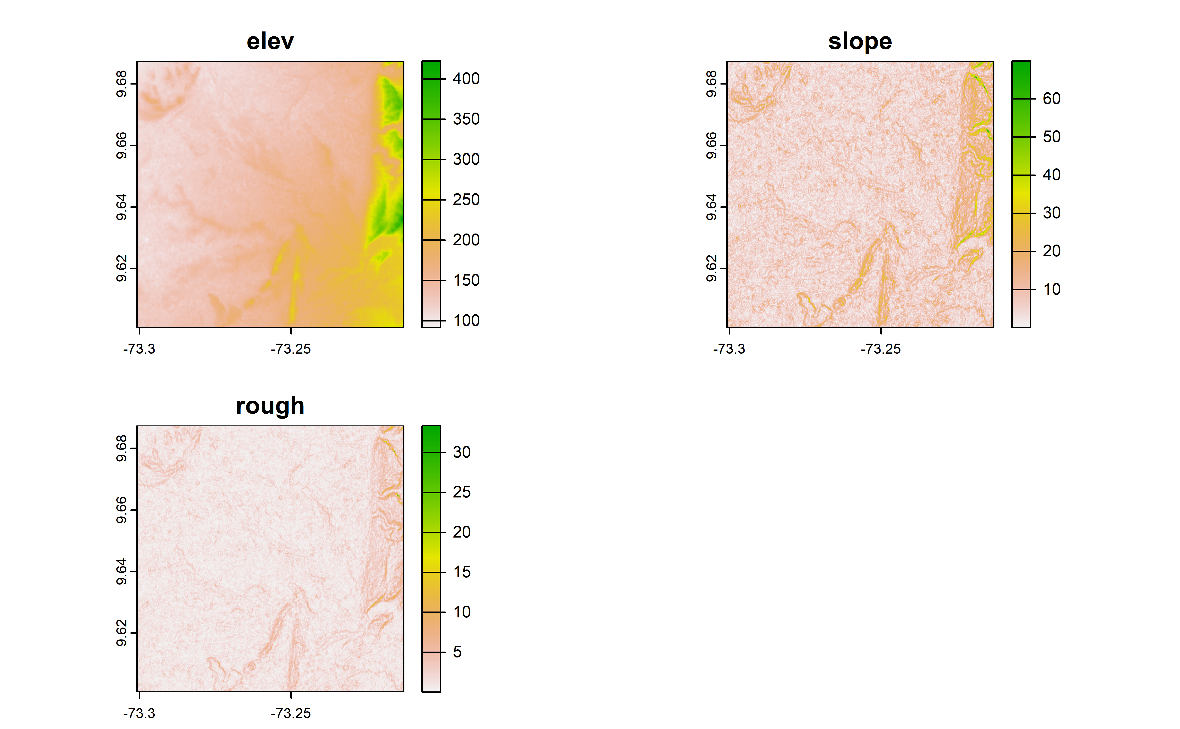
make sf object, get elevation and derive terrain (slope and roughness).

We use the lat and long to make a sf object with the camera locations.

Code

# make sf object
projlatlon <- "+proj=longlat +datum=WGS84 +no_defs +ellps=WGS84 +towgs84=0,0,0"

datos_PCF_sf <-  st_as_sf(x = CToperation,
                         coords = c("Longitude", 
                                    "Latitude"),
                         crs = projlatlon)

# covariates
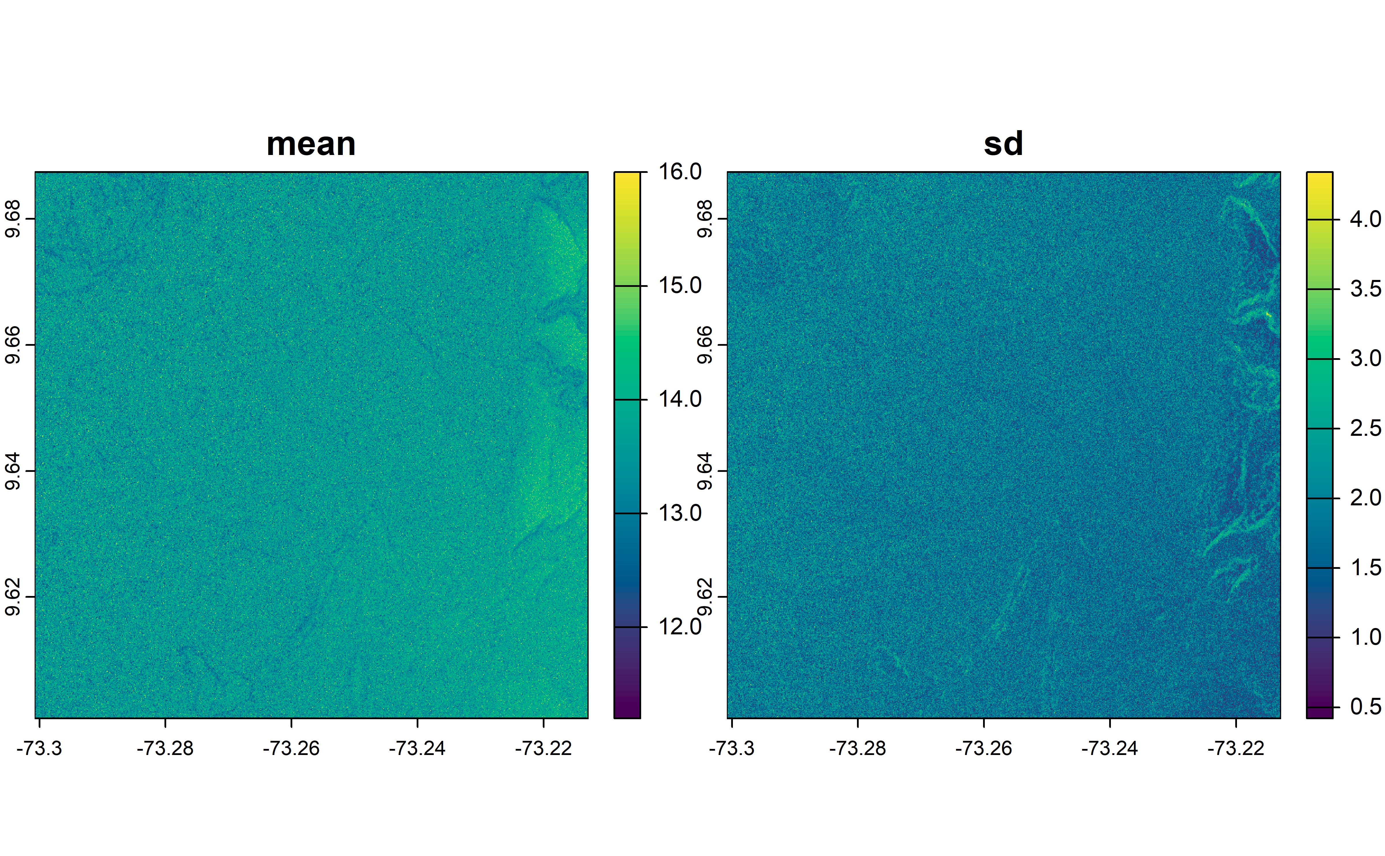
elev <- rast(get_elev_raster(datos_PCF_sf, z=14)) # get raster map
slope <- terrain(elev, v="slope", neighbors=8, unit="degrees")  
# also slope, aspect, TPI, TRI, TRIriley, TRIrmsd, roughness, flowdir 
rough <- terrain(elev, v="roughness", neighbors=8, unit="degrees")  
# landcover <- rast("C:/CodigoR/WCS-CameraTrap/raster/latlon/LandCover_Type_Yearly_500m_v61/LC1/MCD12Q1_LC1_2021_001.tif") 

cos_rast <- c(elev,slope, rough) # make a stack
# rename stack
names(cos_rast) <- c("elev", "slope", "rough")

plot(cos_rast)

Code

mapview(elev) + mapview(datos_PCF_sf)

Extract values from the rasters

We use the camera locations to extract the raster (elevations, slope and roughness) information.

Code


# extract
covs <- terra::extract(cos_rast, datos_PCF_sf)
# landcov <- terra::extract(landcover, datos_PCF_sf)

Multispecies occupancy model

Preparing the model

Now we have all ready to make our model. We put the data of the species, and the covariates in a list.

Code

# check consistancy equal mumner of spatial covariates and rows in data
# identical(nrow(ylist[[1]]), nrow(covars)) 

# Base de datos para los análisis -----------------------------------------

data_list <- list(ylist    = ylist, # Historias de detección
                  siteCovs = covs[,2:4], #covars, # Covariables de sitio
                  obsCovs  = list(effort = DetHist_list[[1]]$effort))  # agregamos el esfuerzo de muestreo como covariable de observación

# 3. 1 Modelo multi-especie  -----------------------------------------

# Se creará un txt temporal donde estarán las especificaciones del modelo en enfoque Bayesiano
modelfile <- (fileext = "modoccu.txt")

# Usaremos la función ` communityModel`

Generating the model

We use the function ‘communityModel’ to setup our model, selecting which covariates is for detection or occupancy and if it is fixed or random effect.

Code


# Generemos el modelo
comu_model <- communityModel(data_list, # la lista de datos
                             occuCovs = list(ranef=c("rough", "elev")), # ranef La covariables de sitio
                             detCovsObservation = list(fixed = "effort"), #Covariables de observación
                             intercepts = list(det = "ranef", occu = "ranef"),
                             augmentation = c(full = 30),# Número aumentado de especies
                             modelFile = "modelfile")

summary(comu_model)
#> commOccu object for community occupancy model (in JAGS)
#> 
#> 30 species,  23 stations,  39 occasions
#> 530 occasions with effort
#> Number of detections (by species): 0 - 164 
#> 
#> Available site covariates:
#>  elev, slope, rough 
#> 
#> Used site covariates:
#>  elev, rough 
#> 
#> Available site-occasion covariates:
#>  effort

Running the model

Go for a coffe and enjoy while you wait for the signal beep.

Code
# Running the model

fit.commu <- fit(comu_model,
                 n.iter = 1200,
                 n.burnin = 200,
                 thin = 2,
                 chains = 3,
                 cores = 3,
                 quiet = T
);beep(sound = 4)

# save the results to not run again
save(fit.commu, file="C:/CodigoR/CameraTrapCesar/posts/2024-06-20-multispecies-occupancy/result/DR_result.R") # guardamos los resultados para no correr de nuevo

See the results

As a table

Code

# Resultados --------------------------------------------------------------

# Extraemos lo tabla de valores estimados
modresult <- as.data.frame(summary(fit.commu)[["statistics"]])
# View(modresult)
DT::datatable(round(summary(fit.commu)$statistics, 3))

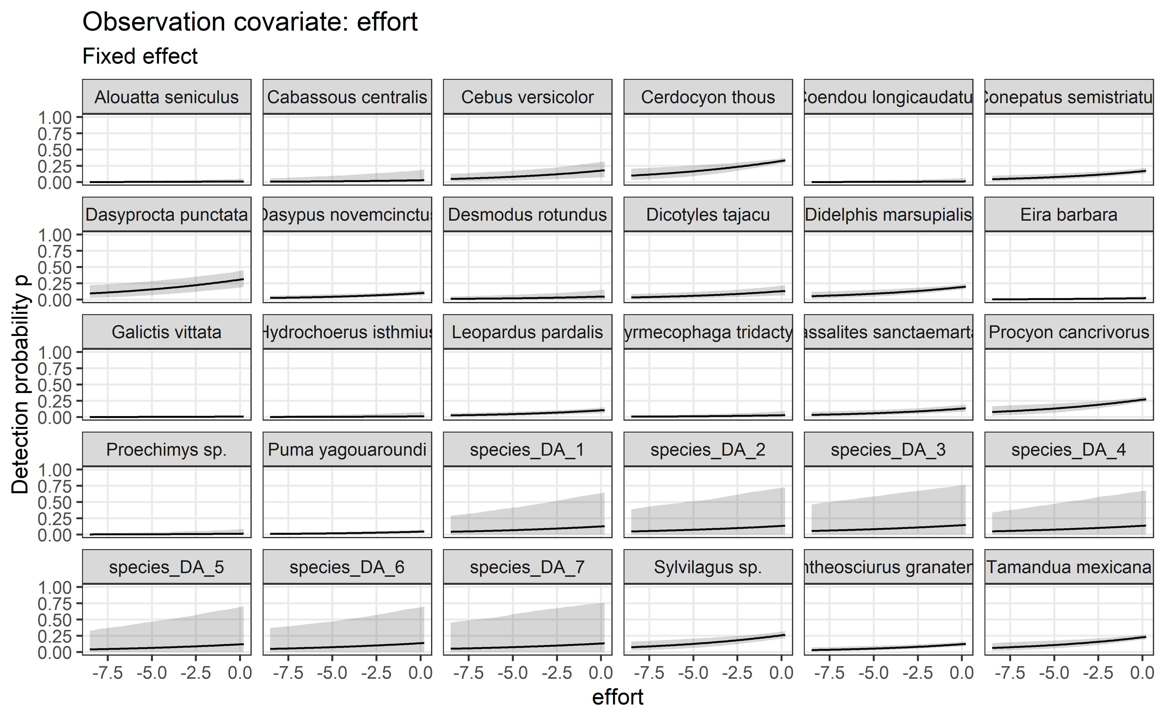
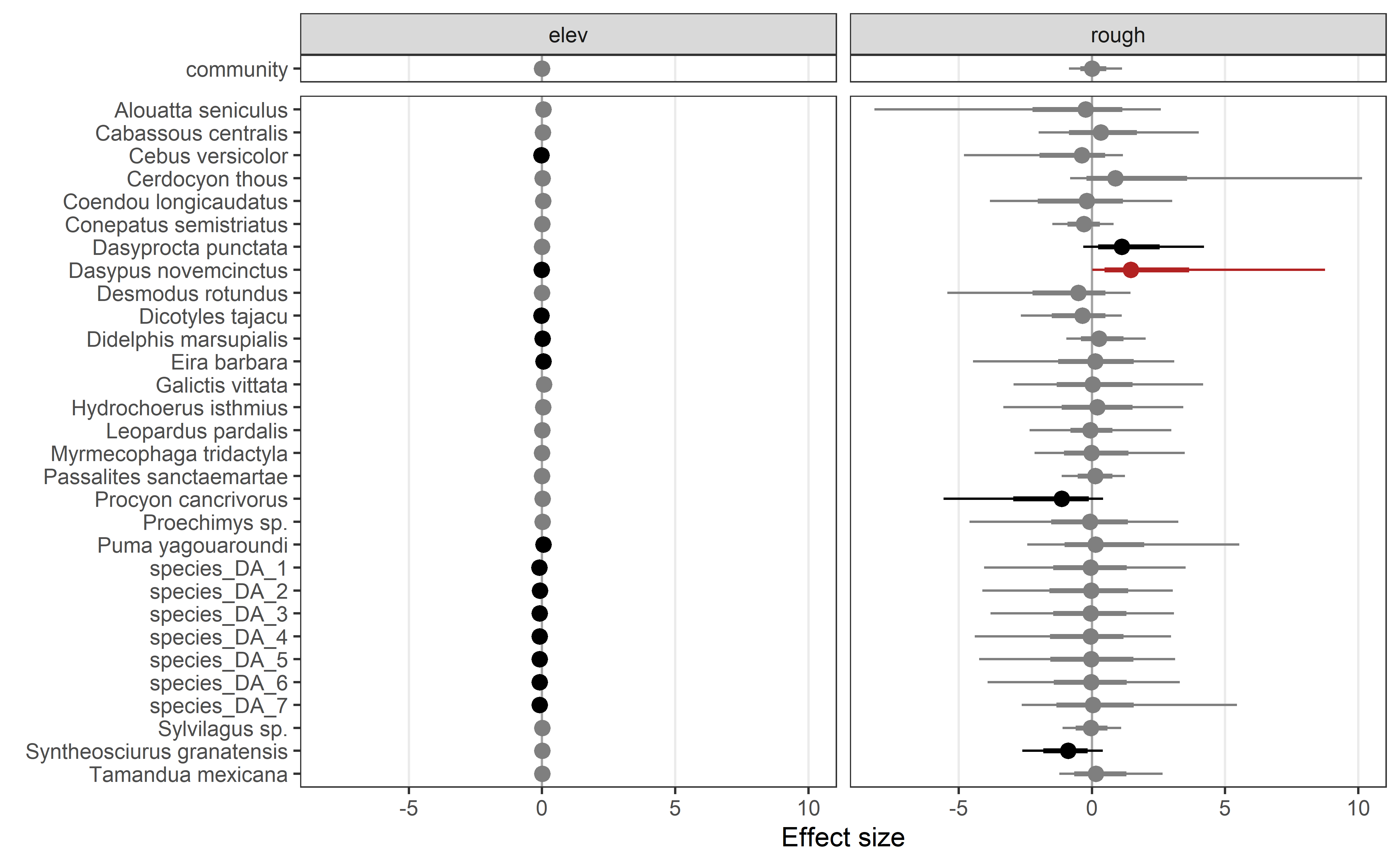
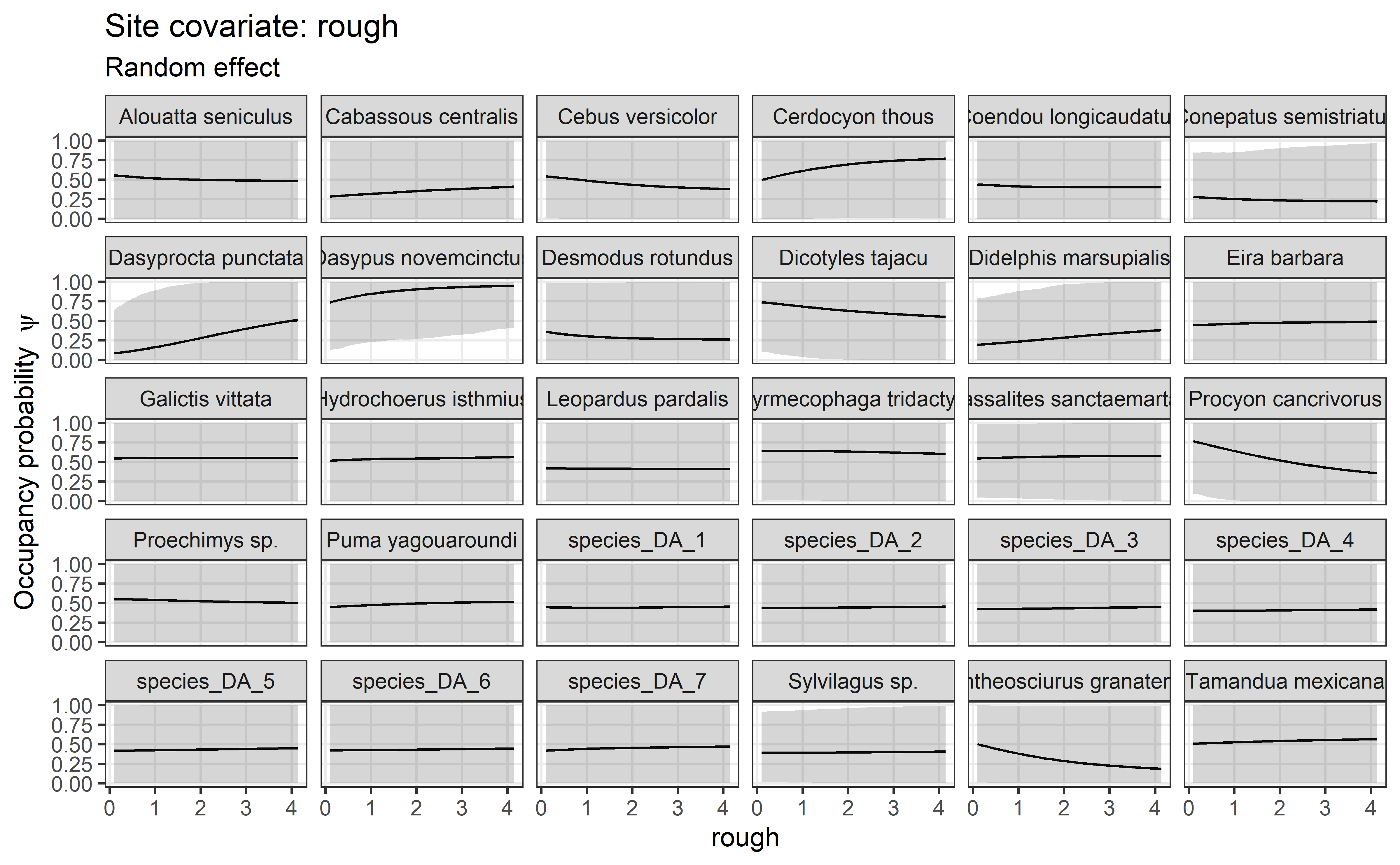
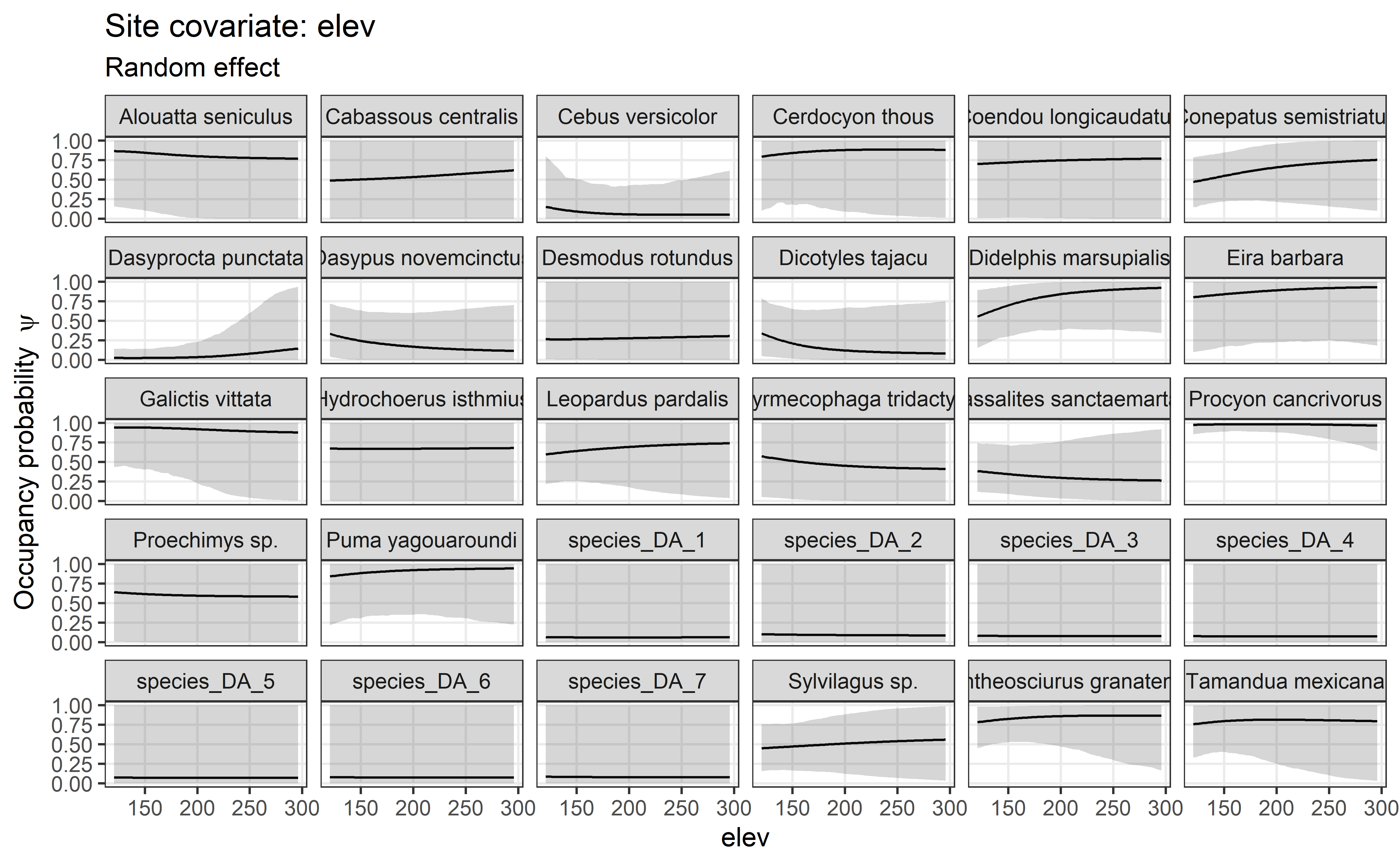
As graphs

Code
# Gráficos de predicción y de coeficientes

# Otra gran ventaja de CamtrapR es que permite gráficar de manera muy sencilla la predicción posterior del modelo. Veamos que pasa con la ocupación de cada especie

plot_effects(comu_model,
              fit.commu,
              submodel = "det")
#> $effort

Code

plot_coef(comu_model,
           fit.commu,
           submodel = "state",
           combine = T)

Code

plot_effects(comu_model, # El modelo
             fit.commu, # El objeto ajustado
             submodel = "state",
             response = "occupancy") # el parámetro de interés
#> $rough

#> 
#> $elev

Code

# Ahora con los coeficientes estimados

# plot_coef(comu_model,
#           fit.commu,
#           submodel = "state")

See the species richness

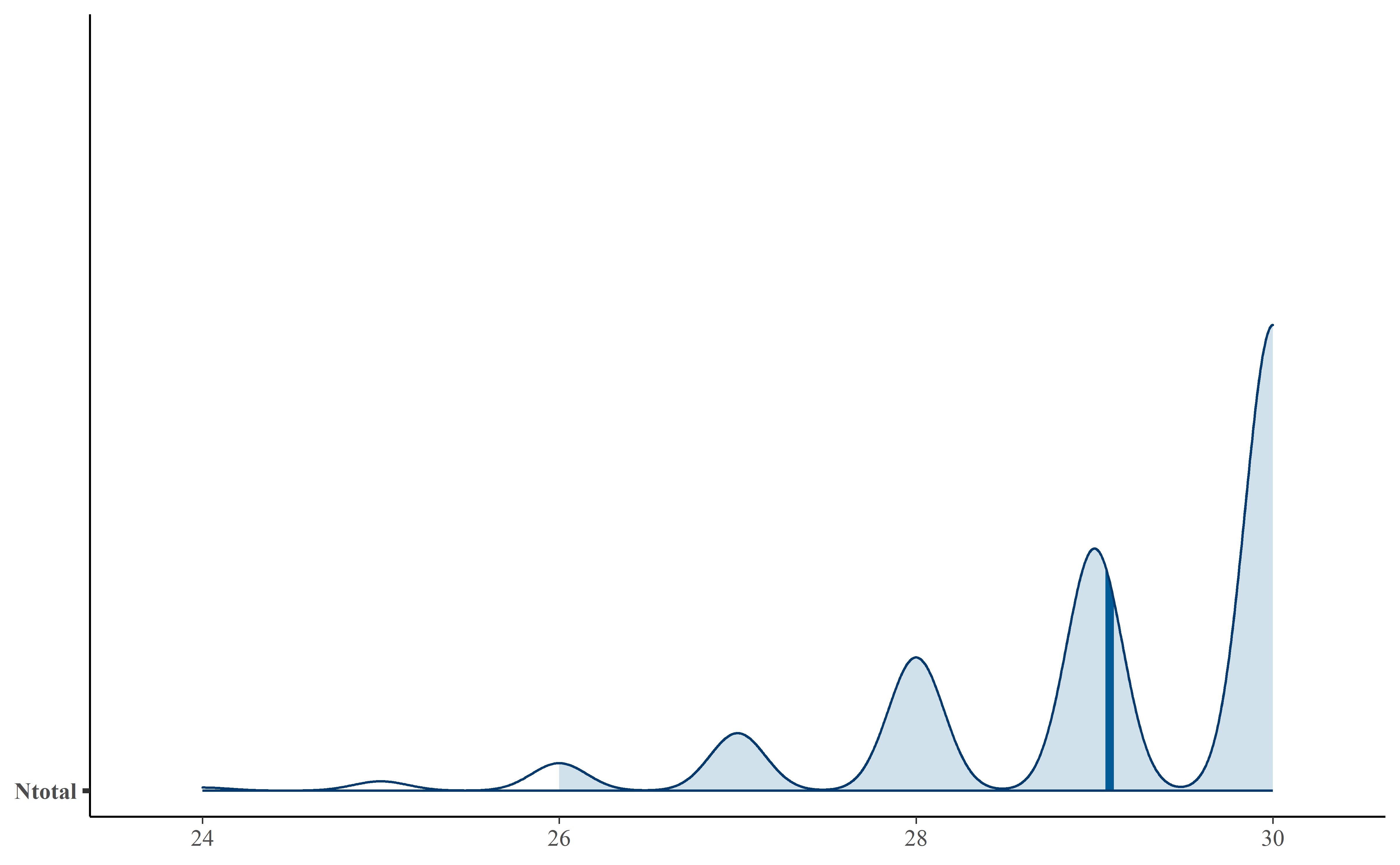
Notice the estimated species richness, Mean, SD, and SE is: 29.0866667, 1.1764686, 0.0303763, 0.0529884

Code

# Valor de Ntotal, es decir del número de especies estimado
(riqueza_est <- modresult["Ntotal",])
#>            Mean       SD   Naive SE Time-series SE
#> Ntotal 29.08667 1.176469 0.03037629     0.05298842

# Veamos el gráfico de la distribución posterior
mcmc_areas(fit.commu, # objeto jags
           pars= "Ntotal", # parámetro de interés
           point_est = "mean",
           prob = 0.95) # intervalos de credibilidad

Code


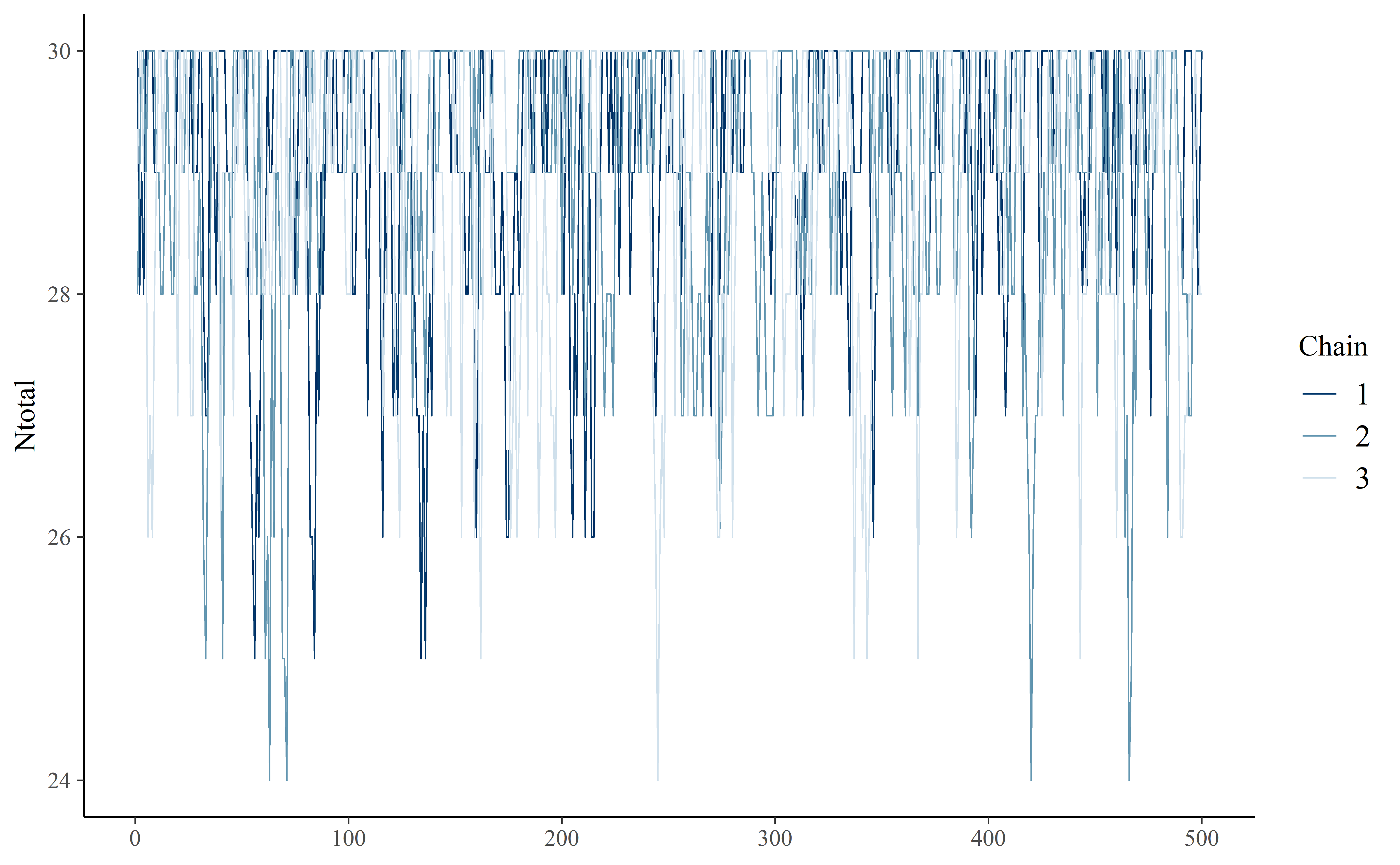
# La estimación no se ve muy bien, hay que verificar los trace plots

mcmc_trace(fit.commu, pars = "Ntotal")

Code

# Debería verse como un cesped, muy probablemente necesitamos muchas mas iteraciones para este modelo

gd <- as.data.frame(gelman.diag(fit.commu,  multivariate = FALSE)[[1]])
DT::datatable(gd["Ntotal",])
Code

#La prueba de Gelman-Rubin debe ser ~1 para considerar que hay buena convergencia. Aunque tenemos un valor bueno para Ntotal, hay varios valores de omega con NA, eso puede estar causando los problemas.

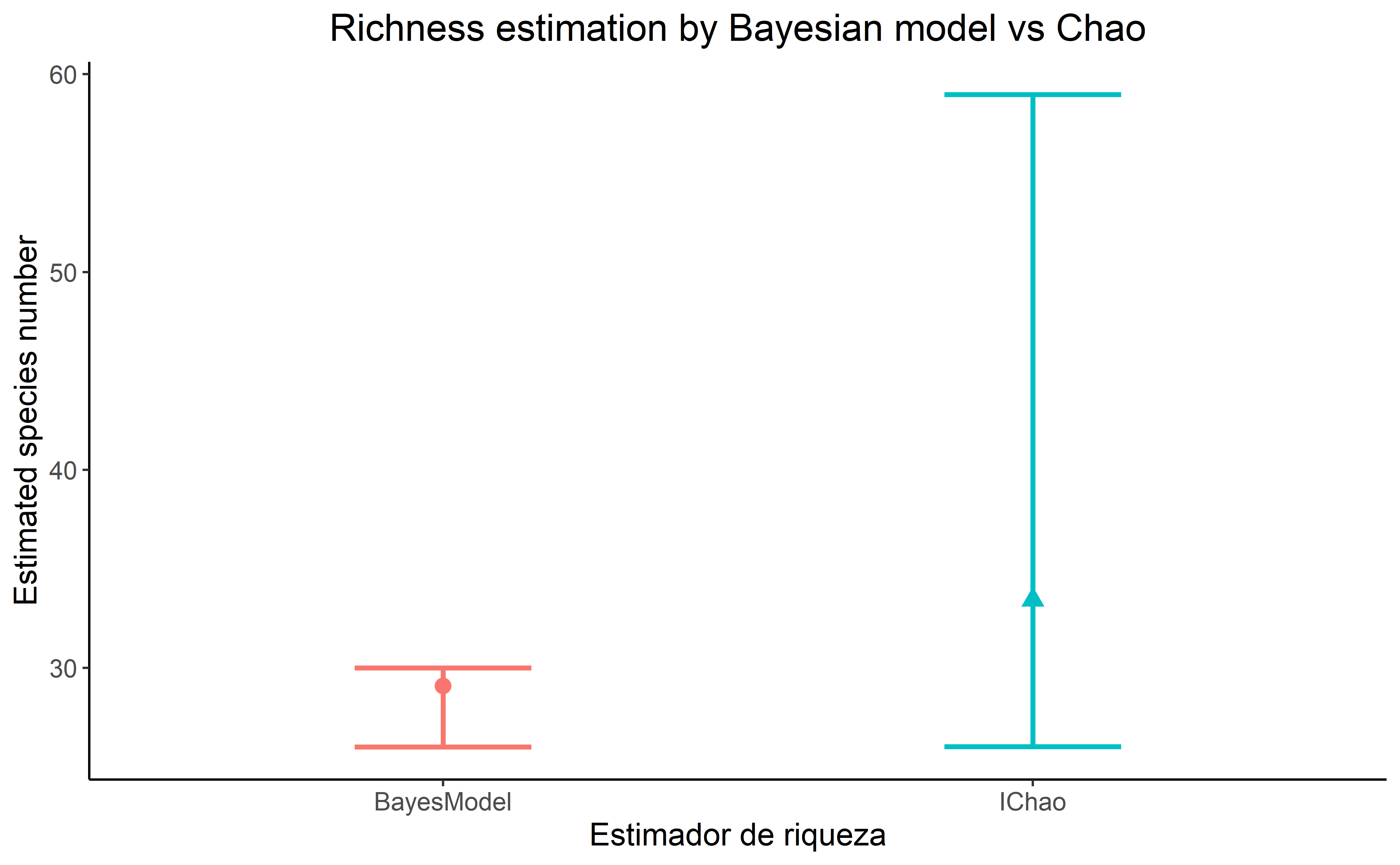
Comparing species richness with Chao

Code

# Comparando con métodos clásicos -----------------------------------------


# Formatear los datos a un vector de frecuencia
inci_Chao <- ylist %>%  # historias de captura
  map(~rowSums(.,na.rm = T)) %>% # sumo las detecciones en cada sitio
  reduce(cbind) %>% # unimos las listas
  t() %>% # trasponer la tabla
  as_tibble() %>% #formato tibble
  mutate_if(is.numeric,~(.>=1)*1) %>%  #como es incidencia, formateo a 1 y 0
  rowSums() %>%  # ahora si la suma de las incidencias en cada sitio
  as_tibble() %>% 
 add_row(value= dim(CToperation)[1], .before = 1) %>%  # el formato requiere que el primer valor sea el número de sitios
  as.matrix() # Requiere formato de matriz


# Calcular la riqueza con estimadores no paramétricos
chao_sp <- ChaoSpecies(inci_Chao, datatype = "incidence_freq")

NIChao <- chao_sp$Species_table[4,c(1,3,4)] # Extraer valores de IChao

Nocu<- mcmc_intervals(fit.commu, pars = "Ntotal", prob = 0.95,prob_outer = 0.99, point_est = "mean")[[1]] %>%  # Extraer valores del bayes plot
  select(m,l,h) %>% # Seleccionar columnas
  rename("Estimate"= m, # Renombrarlas
         "95%Lower"= l,
         "95%Upper"= h)


# Unir en un solo dataframe
Nplotdata <- rbind(IChao=NIChao, BayesModel=Nocu) %>% 
  as.data.frame() %>% 
  rownames_to_column(.)

# Gráfico para comparar la riqueza estimada
plotN <- ggplot(Nplotdata, aes(x=rowname, y= Estimate, col=rowname))+
  geom_point(aes(shape=rowname),size=3)+
  geom_errorbar(aes(ymin= `95%Lower`, ymax= `95%Upper`), width=.3, size=1)+
  labs(x="Estimador de riqueza",y="Estimated species number", title = "Richness estimation by Bayesian model vs Chao")+
  theme_classic()+
  theme(text=element_text(size = 13), plot.title = element_text(hjust= 0.5), legend.position = "none")

plotN

Spatial prediction

Occupancy

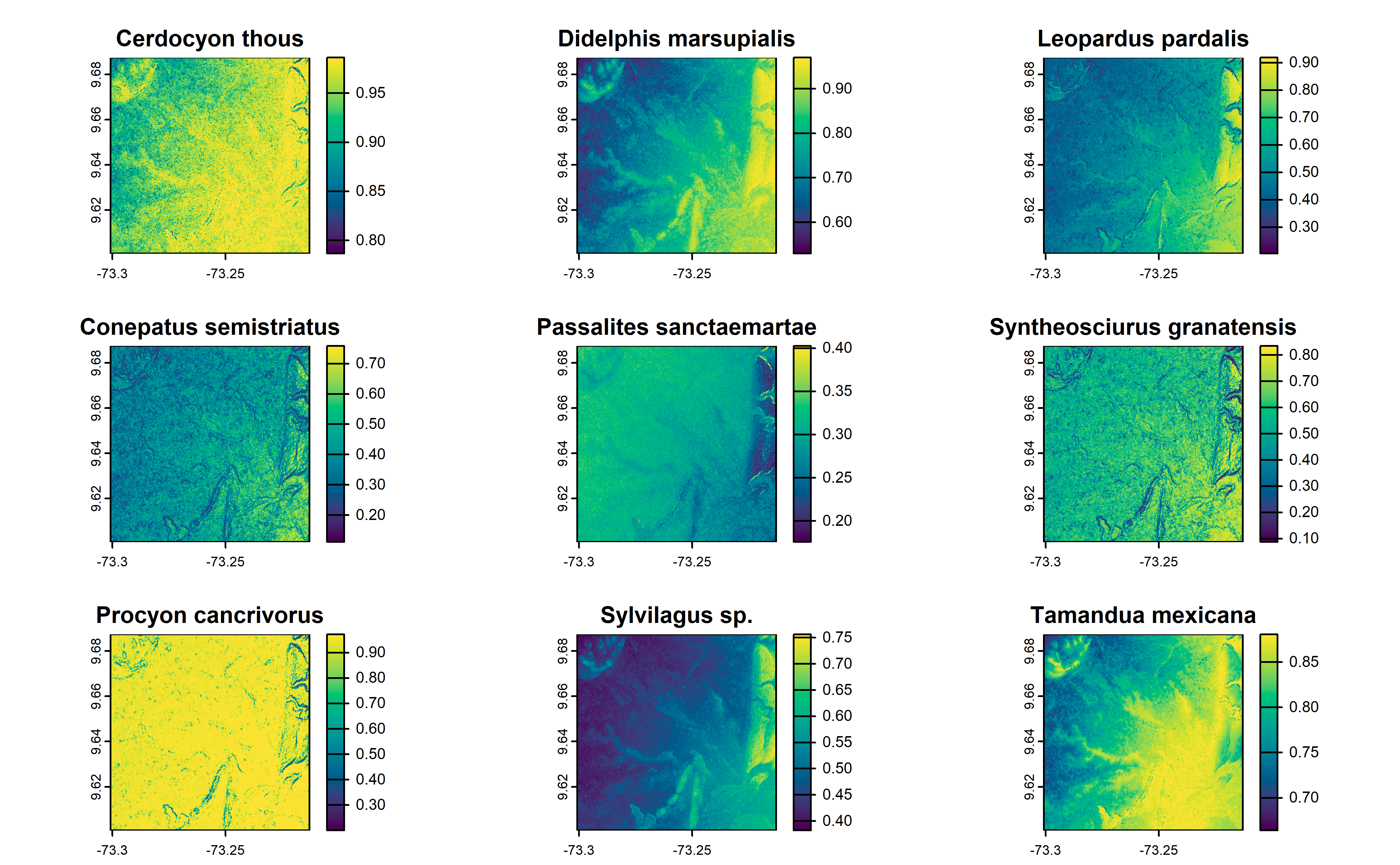
Just like magic camtrapR allow us to make predictions using a raster object, obtaining maps of richness and occupancy per species.

Be aware if you used a large number in interations for better fit in the Running model part, you can get the Error: cannot locate a vector size 467.8 Gb

Here we are plotting only the first 9 species for space reasons.

Code
# species occupancy estimates
predictions_psi <- camtrapR::predict(object    = comu_model, 
                             mcmc.list = fit.commu,
                             x         = cos_rast,
                             type      = "psi",
                             draws     = 1000)

# save the results to not run again
writeRaster(predictions_psi[[1]], file="C:/CodigoR/CameraTrapCesar/posts/2024-06-20-multispecies-occupancy/result/predictions_psi.tif", overwrite=TRUE) # guardamos los resultados para no correr de nuevo


# Plot occupancy
plot(predictions_psi$mean, zlim = c(0,1), 
       col = hcl.colors(100), 
       maxnl = 9,   # plotting only the first 9 species for space reasons
       asp = 1)  
  

Species Richness

Notice this prediction can be also very RAM consuming…

Code
# species richness estimates
predictions_rich <- predict(object   = comu_model, 
                             mcmc.list = fit.commu,
                             x         = cos_rast,
                             type      = "richness",
                            draws     = 1000)

# save the results to not run again
writeRaster(predictions_rich, file="C:/CodigoR/CameraTrapCesar/posts/2024-06-20-multispecies-occupancy/result/predictions_rich.tif") # guardamos los resultados para no correr de nuevo


# plot richness
plot(predictions_rich, col = hcl.colors(100), asp = 1)
  

An additional option to avoid the out of memory issue is to aggregate the pixel size in the raster object before making the prediction.

Code
agregated_raster <- aggregate(old_raster, fact = 10) # aggregate 10 pixels in one

Package Citation

Code
pkgs <- cite_packages(output = "paragraph", out.dir = ".") #knitr::kable(pkgs)
#> WARNING: One or more problems were discovered while enumerating dependencies.
#> 
#> # C:/CodigoR/CameraTrapCesar/posts/2024-06-20-multispecies-occupancy/result/DR_result.R --------
#> Error: invalid multibyte character in parser (<input>:4:4)
#> 
#> # C:/CodigoR/CameraTrapCesar/posts/2024-06-20-multispecies-occupancy/result/predictions_psi.R --------
#> Error: invalid multibyte character in parser (<input>:11:2)
#> 
#> Please see `?renv::dependencies` for more information.
pkgs

We used R version 4.3.2 (R Core Team 2023) and the following R packages: bayesplot v. 1.11.1 (Gabry et al. 2019; Gabry and Mahr 2024), beepr v. 1.3 (Bååth 2018), camtrapR v. 2.3.0 (Niedballa et al. 2016), devtools v. 2.4.5 (Wickham et al. 2022), DT v. 0.32 (Xie, Cheng, and Tan 2024), elevatr v. 0.99.0 (Hollister et al. 2023), kableExtra v. 1.4.0 (Zhu 2024), mapview v. 2.11.2 (Appelhans et al. 2023), nimble v. 1.1.0 (de Valpine et al. 2017, 2024b, 2024a), patchwork v. 1.2.0 (Pedersen 2024), quarto v. 1.4 (Allaire and Dervieux 2024), rjags v. 4.15 (Plummer 2023), rmarkdown v. 2.27 (Xie, Allaire, and Grolemund 2018; Xie, Dervieux, and Riederer 2020; Allaire et al. 2024), sf v. 1.0.15 (Pebesma 2018; Pebesma and Bivand 2023), snowfall v. 1.84.6.3 (Knaus 2023), SpadeR v. 0.1.1 (Chao et al. 2016), styler v. 1.10.3 (Müller and Walthert 2024), terra v. 1.7.71 (Hijmans 2024), tictoc v. 1.2.1 (Izrailev 2024), tidyverse v. 2.0.0 (Wickham et al. 2019).

Sesion info

Session info
#> ─ Session info ───────────────────────────────────────────────────────────────────────────────────────────────────────
#>  setting  value
#>  version  R version 4.3.2 (2023-10-31 ucrt)
#>  os       Windows 10 x64 (build 19042)
#>  system   x86_64, mingw32
#>  ui       RTerm
#>  language (EN)
#>  collate  Spanish_Colombia.utf8
#>  ctype    Spanish_Colombia.utf8
#>  tz       America/Bogota
#>  date     2024-07-04
#>  pandoc   3.1.11 @ C:/Program Files/RStudio/resources/app/bin/quarto/bin/tools/ (via rmarkdown)
#> 
#> ─ Packages ───────────────────────────────────────────────────────────────────────────────────────────────────────────
#>  ! package           * version    date (UTC) lib source
#>    abind               1.4-5      2016-07-21 [1] CRAN (R 4.3.1)
#>    audio               0.1-11     2023-08-18 [1] CRAN (R 4.3.1)
#>    backports           1.4.1      2021-12-13 [1] CRAN (R 4.3.1)
#>    base64enc           0.1-3      2015-07-28 [1] CRAN (R 4.3.1)
#>    bayesplot         * 1.11.1     2024-02-15 [1] CRAN (R 4.3.3)
#>    beepr             * 1.3        2018-06-04 [1] CRAN (R 4.3.3)
#>    brew                1.0-10     2023-12-16 [1] CRAN (R 4.3.2)
#>    bslib               0.6.1      2023-11-28 [1] CRAN (R 4.3.2)
#>    cachem              1.0.8      2023-05-01 [1] CRAN (R 4.3.2)
#>    camtrapR          * 2.3.0      2024-02-26 [1] CRAN (R 4.3.3)
#>    cellranger          1.1.0      2016-07-27 [1] CRAN (R 4.3.2)
#>    checkmate           2.3.1      2023-12-04 [1] CRAN (R 4.3.2)
#>    class               7.3-22     2023-05-03 [2] CRAN (R 4.3.2)
#>    classInt            0.4-10     2023-09-05 [1] CRAN (R 4.3.2)
#>    cli                 3.6.2      2023-12-11 [1] CRAN (R 4.3.2)
#>    coda              * 0.19-4.1   2024-01-31 [1] CRAN (R 4.3.2)
#>    codetools           0.2-19     2023-02-01 [2] CRAN (R 4.3.2)
#>    colorspace          2.1-0      2023-01-23 [1] CRAN (R 4.3.2)
#>    crayon              1.5.2      2022-09-29 [1] CRAN (R 4.3.2)
#>    crosstalk           1.2.1      2023-11-23 [1] CRAN (R 4.3.2)
#>    curl                5.2.0      2023-12-08 [1] CRAN (R 4.3.2)
#>    data.table          1.15.0     2024-01-30 [1] CRAN (R 4.3.2)
#>    DBI                 1.2.2      2024-02-16 [1] CRAN (R 4.3.2)
#>    devtools            2.4.5      2022-10-11 [1] CRAN (R 4.3.2)
#>    digest              0.6.34     2024-01-11 [1] CRAN (R 4.3.2)
#>    distributional      0.4.0      2024-02-07 [1] CRAN (R 4.3.2)
#>    dplyr             * 1.1.4      2023-11-17 [1] CRAN (R 4.3.2)
#>    DT                  0.32       2024-02-19 [1] CRAN (R 4.3.3)
#>    e1071               1.7-14     2023-12-06 [1] CRAN (R 4.3.2)
#>    elevatr           * 0.99.0     2023-09-12 [1] CRAN (R 4.3.2)
#>    ellipsis            0.3.2      2021-04-29 [1] CRAN (R 4.3.2)
#>    evaluate            0.23       2023-11-01 [1] CRAN (R 4.3.2)
#>    fansi               1.0.6      2023-12-08 [1] CRAN (R 4.3.2)
#>    farver              2.1.1      2022-07-06 [1] CRAN (R 4.3.2)
#>    fastmap             1.1.1      2023-02-24 [1] CRAN (R 4.3.2)
#>    forcats           * 1.0.0      2023-01-29 [1] CRAN (R 4.3.2)
#>    fs                  1.6.3      2023-07-20 [1] CRAN (R 4.3.2)
#>    generics            0.1.3      2022-07-05 [1] CRAN (R 4.3.2)
#>    ggplot2           * 3.5.1      2024-04-23 [1] CRAN (R 4.3.3)
#>    ggridges            0.5.6      2024-01-23 [1] CRAN (R 4.3.3)
#>    glue                1.7.0      2024-01-09 [1] CRAN (R 4.3.2)
#>    grateful          * 0.2.4      2023-10-22 [1] CRAN (R 4.3.3)
#>    gtable              0.3.4      2023-08-21 [1] CRAN (R 4.3.2)
#>    hms                 1.1.3      2023-03-21 [1] CRAN (R 4.3.2)
#>    htmltools           0.5.7      2023-11-03 [1] CRAN (R 4.3.2)
#>    htmlwidgets         1.6.4      2023-12-06 [1] CRAN (R 4.3.2)
#>    httpuv              1.6.14     2024-01-26 [1] CRAN (R 4.3.2)
#>    httr                1.4.7      2023-08-15 [1] CRAN (R 4.3.2)
#>    igraph              2.0.2      2024-02-17 [1] CRAN (R 4.3.2)
#>    jquerylib           0.1.4      2021-04-26 [1] CRAN (R 4.3.2)
#>    jsonlite            1.8.8      2023-12-04 [1] CRAN (R 4.3.2)
#>    kableExtra        * 1.4.0      2024-01-24 [1] CRAN (R 4.3.3)
#>    KernSmooth          2.23-22    2023-07-10 [2] CRAN (R 4.3.2)
#>    knitr               1.46       2024-04-06 [1] CRAN (R 4.3.3)
#>    labeling            0.4.3      2023-08-29 [1] CRAN (R 4.3.1)
#>    later               1.3.2      2023-12-06 [1] CRAN (R 4.3.2)
#>    lattice             0.22-5     2023-10-24 [1] CRAN (R 4.3.2)
#>    leafem              0.2.3      2023-09-17 [1] CRAN (R 4.3.2)
#>    leaflet             2.2.1      2023-11-13 [1] CRAN (R 4.3.2)
#>    leaflet.providers   2.0.0      2023-10-17 [1] CRAN (R 4.3.2)
#>    leafpop             0.1.0      2021-05-22 [1] CRAN (R 4.3.2)
#>    lifecycle           1.0.4      2023-11-07 [1] CRAN (R 4.3.2)
#>    lubridate         * 1.9.3      2023-09-27 [1] CRAN (R 4.3.2)
#>    lwgeom              0.2-13     2023-05-22 [1] CRAN (R 4.3.2)
#>    magrittr            2.0.3      2022-03-30 [1] CRAN (R 4.3.2)
#>    mapview           * 2.11.2     2023-10-13 [1] CRAN (R 4.3.2)
#>    MASS                7.3-60     2023-05-04 [2] CRAN (R 4.3.2)
#>    Matrix              1.6-1.1    2023-09-18 [2] CRAN (R 4.3.2)
#>    memoise             2.0.1      2021-11-26 [1] CRAN (R 4.3.2)
#>    mgcv                1.9-1      2023-12-21 [1] CRAN (R 4.3.3)
#>    mime                0.12       2021-09-28 [1] CRAN (R 4.3.1)
#>    miniUI              0.1.1.1    2018-05-18 [1] CRAN (R 4.3.2)
#>    munsell             0.5.0      2018-06-12 [1] CRAN (R 4.3.2)
#>    nimble            * 1.1.0      2024-01-31 [1] CRAN (R 4.3.3)
#>    nlme                3.1-163    2023-08-09 [2] CRAN (R 4.3.2)
#>    numDeriv            2016.8-1.1 2019-06-06 [1] CRAN (R 4.3.1)
#>    patchwork         * 1.2.0      2024-01-08 [1] CRAN (R 4.3.3)
#>    pillar              1.9.0      2023-03-22 [1] CRAN (R 4.3.2)
#>    pkgbuild            1.4.4      2024-03-17 [1] CRAN (R 4.3.3)
#>    pkgconfig           2.0.3      2019-09-22 [1] CRAN (R 4.3.2)
#>    pkgload             1.3.4      2024-01-16 [1] CRAN (R 4.3.2)
#>    plyr                1.8.9      2023-10-02 [1] CRAN (R 4.3.2)
#>    png                 0.1-8      2022-11-29 [1] CRAN (R 4.3.1)
#>    posterior           1.5.0      2023-10-31 [1] CRAN (R 4.3.2)
#>    pracma              2.4.4      2023-11-10 [1] CRAN (R 4.3.3)
#>    prettyunits         1.2.0      2023-09-24 [1] CRAN (R 4.3.2)
#>    processx            3.8.3      2023-12-10 [1] CRAN (R 4.3.2)
#>    profvis             0.3.8      2023-05-02 [1] CRAN (R 4.3.2)
#>    progress            1.2.3      2023-12-06 [1] CRAN (R 4.3.3)
#>    progressr           0.14.0     2023-08-10 [1] CRAN (R 4.3.2)
#>    promises            1.2.1      2023-08-10 [1] CRAN (R 4.3.2)
#>    proxy               0.4-27     2022-06-09 [1] CRAN (R 4.3.2)
#>    ps                  1.7.6      2024-01-18 [1] CRAN (R 4.3.2)
#>    purrr             * 1.0.2      2023-08-10 [1] CRAN (R 4.3.2)
#>    quarto            * 1.4        2024-03-06 [1] CRAN (R 4.3.3)
#>    R.cache             0.16.0     2022-07-21 [1] CRAN (R 4.3.3)
#>    R.methodsS3         1.8.2      2022-06-13 [1] CRAN (R 4.3.3)
#>    R.oo                1.26.0     2024-01-24 [1] CRAN (R 4.3.3)
#>    R.utils             2.12.3     2023-11-18 [1] CRAN (R 4.3.3)
#>    R6                  2.5.1      2021-08-19 [1] CRAN (R 4.3.2)
#>    raster              3.6-26     2023-10-14 [1] CRAN (R 4.3.2)
#>    RColorBrewer        1.1-3      2022-04-03 [1] CRAN (R 4.3.1)
#>    Rcpp                1.0.12     2024-01-09 [1] CRAN (R 4.3.2)
#>    RcppNumerical       0.6-0      2023-09-06 [1] CRAN (R 4.3.3)
#>  D RcppParallel        5.1.7      2023-02-27 [1] CRAN (R 4.3.2)
#>    readr             * 2.1.5      2024-01-10 [1] CRAN (R 4.3.2)
#>    readxl            * 1.4.3      2023-07-06 [1] CRAN (R 4.3.2)
#>    remotes             2.5.0      2024-03-17 [1] CRAN (R 4.3.3)
#>    renv                1.0.7      2024-04-11 [1] CRAN (R 4.3.3)
#>    reshape2            1.4.4      2020-04-09 [1] CRAN (R 4.3.3)
#>    rjags             * 4-15       2023-11-30 [1] CRAN (R 4.3.3)
#>    rlang               1.1.3      2024-01-10 [1] CRAN (R 4.3.2)
#>    rmarkdown           2.27       2024-05-17 [1] CRAN (R 4.3.3)
#>    rstudioapi          0.16.0     2024-03-24 [1] CRAN (R 4.3.3)
#>    s2                  1.1.6      2023-12-19 [1] CRAN (R 4.3.2)
#>    sass                0.4.8      2023-12-06 [1] CRAN (R 4.3.2)
#>    satellite           1.0.5      2024-02-10 [1] CRAN (R 4.3.2)
#>    scales              1.3.0      2023-11-28 [1] CRAN (R 4.3.3)
#>    secr                4.6.6      2024-02-29 [1] CRAN (R 4.3.3)
#>    sessioninfo         1.2.2      2021-12-06 [1] CRAN (R 4.3.2)
#>    sf                * 1.0-15     2023-12-18 [1] CRAN (R 4.3.2)
#>    shiny               1.8.0      2023-11-17 [1] CRAN (R 4.3.2)
#>    slippymath          0.3.1      2019-06-28 [1] CRAN (R 4.3.2)
#>    snow              * 0.4-4      2021-10-27 [1] CRAN (R 4.3.2)
#>    snowfall          * 1.84-6.3   2023-11-26 [1] CRAN (R 4.3.2)
#>    sp                  2.1-3      2024-01-30 [1] CRAN (R 4.3.2)
#>    SpadeR            * 0.1.1      2016-09-06 [1] CRAN (R 4.3.1)
#>    stars               0.6-4      2023-09-11 [1] CRAN (R 4.3.2)
#>    stringi             1.8.3      2023-12-11 [1] CRAN (R 4.3.2)
#>    stringr           * 1.5.1      2023-11-14 [1] CRAN (R 4.3.2)
#>    styler            * 1.10.3     2024-04-07 [1] CRAN (R 4.3.3)
#>    svglite             2.1.3      2023-12-08 [1] CRAN (R 4.3.2)
#>    systemfonts         1.0.5      2023-10-09 [1] CRAN (R 4.3.2)
#>    tensorA             0.36.2.1   2023-12-13 [1] CRAN (R 4.3.2)
#>    terra             * 1.7-71     2024-01-31 [1] CRAN (R 4.3.2)
#>    tibble            * 3.2.1      2023-03-20 [1] CRAN (R 4.3.2)
#>    tictoc            * 1.2.1      2024-03-18 [1] CRAN (R 4.3.3)
#>    tidyr             * 1.3.1      2024-01-24 [1] CRAN (R 4.3.2)
#>    tidyselect          1.2.1      2024-03-11 [1] CRAN (R 4.3.3)
#>    tidyverse         * 2.0.0      2023-02-22 [1] CRAN (R 4.3.2)
#>    timechange          0.3.0      2024-01-18 [1] CRAN (R 4.3.2)
#>    tzdb                0.4.0      2023-05-12 [1] CRAN (R 4.3.2)
#>    units               0.8-5      2023-11-28 [1] CRAN (R 4.3.2)
#>    urlchecker          1.0.1      2021-11-30 [1] CRAN (R 4.3.2)
#>    usethis             2.2.3      2024-02-19 [1] CRAN (R 4.3.2)
#>    utf8                1.2.4      2023-10-22 [1] CRAN (R 4.3.2)
#>    uuid                1.2-0      2024-01-14 [1] CRAN (R 4.3.2)
#>    vctrs               0.6.5      2023-12-01 [1] CRAN (R 4.3.2)
#>    viridisLite         0.4.2      2023-05-02 [1] CRAN (R 4.3.2)
#>    withr               3.0.0      2024-01-16 [1] CRAN (R 4.3.2)
#>    wk                  0.9.1      2023-11-29 [1] CRAN (R 4.3.2)
#>    xfun                0.44       2024-05-15 [1] CRAN (R 4.3.3)
#>    xml2                1.3.6      2023-12-04 [1] CRAN (R 4.3.2)
#>    xtable              1.8-4      2019-04-21 [1] CRAN (R 4.3.2)
#>    yaml                2.3.8      2023-12-11 [1] CRAN (R 4.3.2)
#> 
#>  [1] C:/Users/usuario/AppData/Local/R/win-library/4.3
#>  [2] C:/Program Files/R/R-4.3.2/library
#> 
#>  D ── DLL MD5 mismatch, broken installation.
#> 
#> ──────────────────────────────────────────────────────────────────────────────────────────────────────────────────────

References

Allaire, JJ, and Christophe Dervieux. 2024. quarto: R Interface to Quarto Markdown Publishing System. https://CRAN.R-project.org/package=quarto.
Allaire, JJ, Yihui Xie, Christophe Dervieux, Jonathan McPherson, Javier Luraschi, Kevin Ushey, Aron Atkins, et al. 2024. rmarkdown: Dynamic Documents for r. https://github.com/rstudio/rmarkdown.
Appelhans, Tim, Florian Detsch, Christoph Reudenbach, and Stefan Woellauer. 2023. mapview: Interactive Viewing of Spatial Data in r. https://CRAN.R-project.org/package=mapview.
Bååth, Rasmus. 2018. beepr: Easily Play Notification Sounds on Any Platform. https://CRAN.R-project.org/package=beepr.
Chao, Anne, K. H. Ma, T. C. Hsieh, and Chun-Huo Chiu. 2016. SpadeR: Species-Richness Prediction and Diversity Estimation with r. https://CRAN.R-project.org/package=SpadeR.
de Valpine, Perry, Christopher Paciorek, Daniel Turek, Nick Michaud, Cliff Anderson-Bergman, Fritz Obermeyer, Claudia Wehrhahn Cortes, Abel Rodrìguez, Duncan Temple Lang, and Sally Paganin. 2024a. NIMBLE User Manual (version 1.1.0). https://doi.org/10.5281/zenodo.1211190.
———. 2024b. NIMBLE: MCMC, Particle Filtering, and Programmable Hierarchical Modeling (version 1.1.0). https://doi.org/10.5281/zenodo.1211190.
de Valpine, Perry, Daniel Turek, Christopher Paciorek, Cliff Anderson-Bergman, Duncan Temple Lang, and Ras Bodik. 2017. “Programming with Models: Writing Statistical Algorithms for General Model Structures with NIMBLE.” Journal of Computational and Graphical Statistics 26: 403–13. https://doi.org/10.1080/10618600.2016.1172487.
Gabry, Jonah, and Tristan Mahr. 2024. bayesplot: Plotting for Bayesian Models.” https://mc-stan.org/bayesplot/.
Gabry, Jonah, Daniel Simpson, Aki Vehtari, Michael Betancourt, and Andrew Gelman. 2019. “Visualization in Bayesian Workflow.” J. R. Stat. Soc. A 182: 389–402. https://doi.org/10.1111/rssa.12378.
Hijmans, Robert J. 2024. terra: Spatial Data Analysis. https://CRAN.R-project.org/package=terra.
Hollister, Jeffrey, Tarak Shah, Jakub Nowosad, Alec L. Robitaille, Marcus W. Beck, and Mike Johnson. 2023. elevatr: Access Elevation Data from Various APIs. https://doi.org/10.5281/zenodo.8335450.
Izrailev, Sergei. 2024. tictoc: Functions for Timing r Scripts, as Well as Implementations of Stack and StackList Structures. https://CRAN.R-project.org/package=tictoc.
Knaus, Jochen. 2023. snowfall: Easier Cluster Computing (Based on snow). https://CRAN.R-project.org/package=snowfall.
Müller, Kirill, and Lorenz Walthert. 2024. styler: Non-Invasive Pretty Printing of r Code. https://CRAN.R-project.org/package=styler.
Niedballa, Jürgen, Rahel Sollmann, Alexandre Courtiol, and Andreas Wilting. 2016. camtrapR: An r Package for Efficient Camera Trap Data Management.” Methods in Ecology and Evolution 7 (12): 1457–62. https://doi.org/10.1111/2041-210X.12600.
Pebesma, Edzer. 2018. Simple Features for R: Standardized Support for Spatial Vector Data.” The R Journal 10 (1): 439–46. https://doi.org/10.32614/RJ-2018-009.
Pebesma, Edzer, and Roger Bivand. 2023. Spatial Data Science: With applications in R. Chapman and Hall/CRC. https://doi.org/10.1201/9780429459016.
Pedersen, Thomas Lin. 2024. patchwork: The Composer of Plots. https://CRAN.R-project.org/package=patchwork.
Plummer, Martyn. 2023. rjags: Bayesian Graphical Models Using MCMC. https://CRAN.R-project.org/package=rjags.
R Core Team. 2023. R: A Language and Environment for Statistical Computing. Vienna, Austria: R Foundation for Statistical Computing. https://www.R-project.org/.
Wickham, Hadley, Mara Averick, Jennifer Bryan, Winston Chang, Lucy D’Agostino McGowan, Romain François, Garrett Grolemund, et al. 2019. “Welcome to the tidyverse.” Journal of Open Source Software 4 (43): 1686. https://doi.org/10.21105/joss.01686.
Wickham, Hadley, Jim Hester, Winston Chang, and Jennifer Bryan. 2022. devtools: Tools to Make Developing r Packages Easier. https://CRAN.R-project.org/package=devtools.
Xie, Yihui, J. J. Allaire, and Garrett Grolemund. 2018. R Markdown: The Definitive Guide. Boca Raton, Florida: Chapman; Hall/CRC. https://bookdown.org/yihui/rmarkdown.
Xie, Yihui, Joe Cheng, and Xianying Tan. 2024. DT: A Wrapper of the JavaScript Library DataTables. https://CRAN.R-project.org/package=DT.
Xie, Yihui, Christophe Dervieux, and Emily Riederer. 2020. R Markdown Cookbook. Boca Raton, Florida: Chapman; Hall/CRC. https://bookdown.org/yihui/rmarkdown-cookbook.
Zhu, Hao. 2024. kableExtra: Construct Complex Table with kable and Pipe Syntax. https://CRAN.R-project.org/package=kableExtra.

Citation

BibTeX citation:
@online{j._lizcano2024,
  author = {J. Lizcano, Diego},
  title = {Multispecies Occupancy Model},
  date = {2024-06-23},
  url = {https://dlizcano.github.io/cametrapcesar/posts/2024-06-20-multispecies-occupancy/},
  langid = {en}
}
For attribution, please cite this work as:
J. Lizcano, Diego. 2024. “Multispecies Occupancy Model.” June 23, 2024. https://dlizcano.github.io/cametrapcesar/posts/2024-06-20-multispecies-occupancy/.