Species accumulation curves, rarefaction and other plots
using packages vegan and iNext to analyze diversity on camera trap data
R
diversity
accumulation
effort
Author
Affiliation
Diego J. Lizcano
WildMon
Published
June 25, 2024
Species richness and sampling effort
There are two commonly used ways to account for survey effort when estimating species richness using camera traps:
using the rarefaction of observed richness.
using multispecies occupancy models to account for the species present but not observed (occupancy model, taking in to account imperfect detection).
In this post we can see an example of No 1. using the classical approach of community ecology using the vegan package. The vegan package (https://cran.r-project.org/package=vegan) provides tools for descriptive community ecology. It has basic functions of diversity analysis, community ordination and dissimilarity analysis. The vegan package provides most standard tools of descriptive community analysis. Later in the post we carry out another diversity analysis using functions of the package iNEXT.
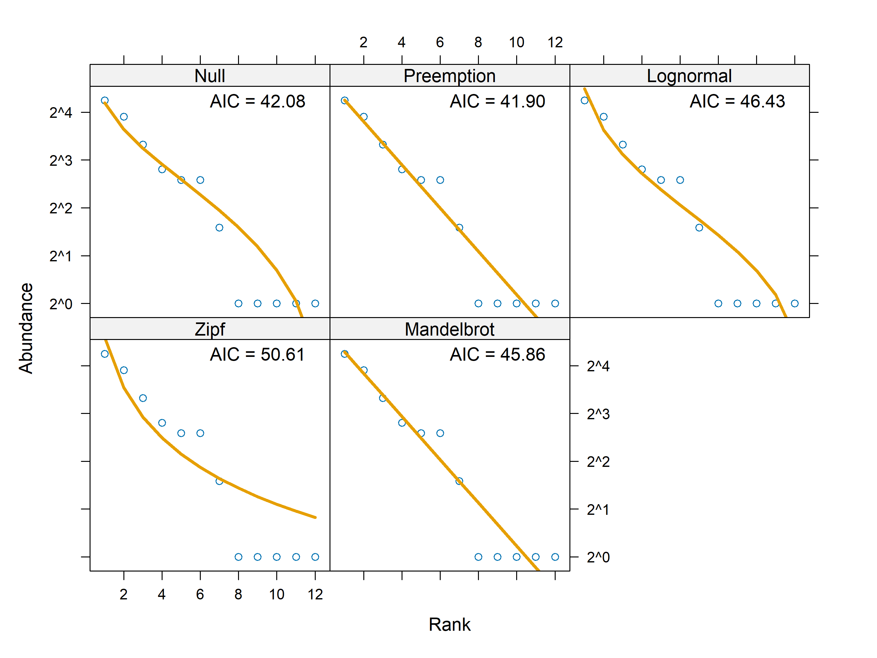
The modern approach to measure species diversity include the “Sample Hill diversities” also known as Hill numbers. Rarefaction and extrapolation with Hill numbers have gain popularity in the last decade and can be computed using the function renyi in the R package vegan (Oksanen 2016) and the function rarity in the R package MeanRarity (Roswell and Dushoff 2020), and Hill diversities of equal-sized or equal-coverage samples can be approximately compared using the functions iNEXT and estimateD in the R package iNEXT (Hsieh et al. 2016). Estimates for asymptotic values of Hill diversity are available in SpadeR (Chao and Jost 2015, Chao et al. 2015).
datos<-read_excel("C:/CodigoR/CameraTrapCesar/data/CT_Cesar.xlsx")# habitat types extracted from Copernicushabs<-read.csv("C:/CodigoR/CameraTrapCesar/data/habitats.csv")
Pooling together several sites
For this example I used data gathered by fundación Galictis in Perija, Colombia. I selected one year for the sites: Becerril 2021, LaPaz_Manaure 2019, MLJ, CL1, CL2 and PCF. Sometimes we need to make unique codes per camera and cameraOperation table. This was not the case.
For this example we are using the habitat type were the camera was installed as a way to see the sampling effort (number of cameras) per habitat type. The habitat type was extracted overlaying the camera points on top of the Land Cover 100m global dataset from COPERNICUS using Google Earth engine connected to R. How to do this will be in another post.
Code
# make a new column Station# datos_PCF <- datos |> dplyr::filter(Proyecto=="CT_LaPaz_Manaure") |> unite ("Station", ProyectoEtapa:Salida:CT, sep = "-")# fix datesdatos$Start<-as.Date(datos$Start, "%d/%m/%Y")datos$End<-as.Date(datos$End, "%d/%m/%Y")datos$eventDate<-as.Date(datos$eventDate, "%d/%m/%Y")datos$eventDateTime<-ymd_hms(paste(datos$eventDate, " ",datos$eventTime, ":00", sep=""))# filter Becerrildatos_Becerril<-datos|>dplyr::filter(ProyectoEtapa=="CT_Becerril")|>mutate(Station=IdGeo)|>filter(Year==2021)# filter LaPaz_Manauredatos_LaPaz_Manaure<-datos|>dplyr::filter(ProyectoEtapa=="CT_LaPaz_Manaure")|>mutate(Station=IdGeo)|>filter(Year==2019)# filter MLJdatos_MLJ<-datos|>dplyr::filter(ProyectoEtapa=="MLJ_TH_TS_2021")|>mutate(Station=IdGeo)# filter CLdatos_CL1<-datos|>dplyr::filter(ProyectoEtapa=="CL-TH2022")|>mutate(Station=IdGeo)# filter CLdatos_CL2<-datos|>dplyr::filter(ProyectoEtapa=="CL-TS2022")|>mutate(Station=IdGeo)# filter PCFdatos_PCF<-datos|>dplyr::filter(Proyecto=="PCF")|>mutate(Station=IdGeo)data_south<-rbind(datos_LaPaz_Manaure, datos_Becerril, datos_MLJ,datos_CL1, datos_CL2,datos_PCF)# filter 2021 and make uniquesCToperation<-data_south|># filter(Year==2021) |> group_by(Station)|>mutate(minStart=min(Start), maxEnd=max(End))|>distinct(Longitude, Latitude, minStart, maxEnd, Year)|>ungroup()
Generating the cameraOperation table and making detection histories for all the species.
The package CamtrapR has the function ‘cameraOperation’ which makes a table of cameras (stations) and dates (setup, puck-up), this table is key to generate the detection histories using the function ‘detectionHistory’ in the next step.
Code
# Generamos la matríz de operación de las cámarascamop<-cameraOperation(CTtable=CToperation, # Tabla de operación stationCol="Station", # Columna que define la estación setupCol="minStart", #Columna fecha de colocación retrievalCol="maxEnd", #Columna fecha de retiro#hasProblems= T, # Hubo fallos de cámaras dateFormat="%Y-%m-%d")#, # Formato de las fechas#cameraCol="CT")# sessionCol= "Year")# Generar las historias de detección ---------------------------------------## remove plroblem species# ind <- which(datos_PCF$Species=="Marmosa sp.")# datos_PCF <- datos_PCF[-ind,]DetHist_list<-lapply(unique(data_south$Species), FUN =function(x){detectionHistory( recordTable =data_south, # Tabla de registros camOp =camop, # Matriz de operación de cámaras stationCol ="Station", speciesCol ="Species", recordDateTimeCol ="eventDateTime", recordDateTimeFormat ="%Y-%m-%d", species =x, # la función reemplaza x por cada una de las especies occasionLength =7, # Colapso de las historias a 10 días day1 ="station", # ("survey"),or #inicia en la fecha de cada station datesAsOccasionNames =FALSE, includeEffort =TRUE, scaleEffort =FALSE, output =("binary"), # ("binary") or ("count")#unmarkedMultFrameInput=TRUE timeZone ="America/Bogota")})# put names to the species names(DetHist_list)<-unique(data_south$Species)# Finally we make a new list to put all the detection histories.ylist<-lapply(DetHist_list, FUN =function(x)x$detection_history)
Use the detection histories to make the a matrix for vegan and the incidence for iNEXT.
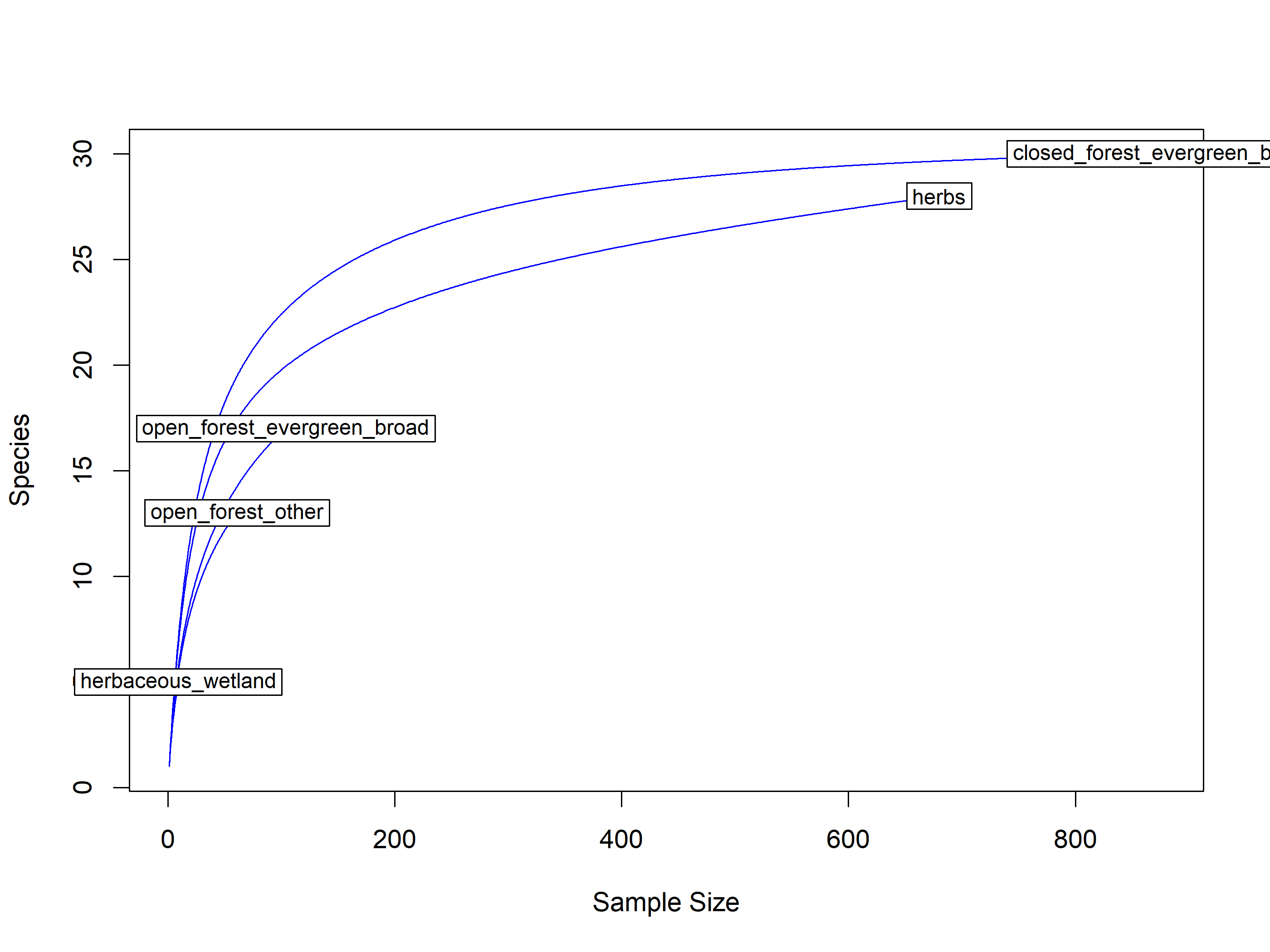
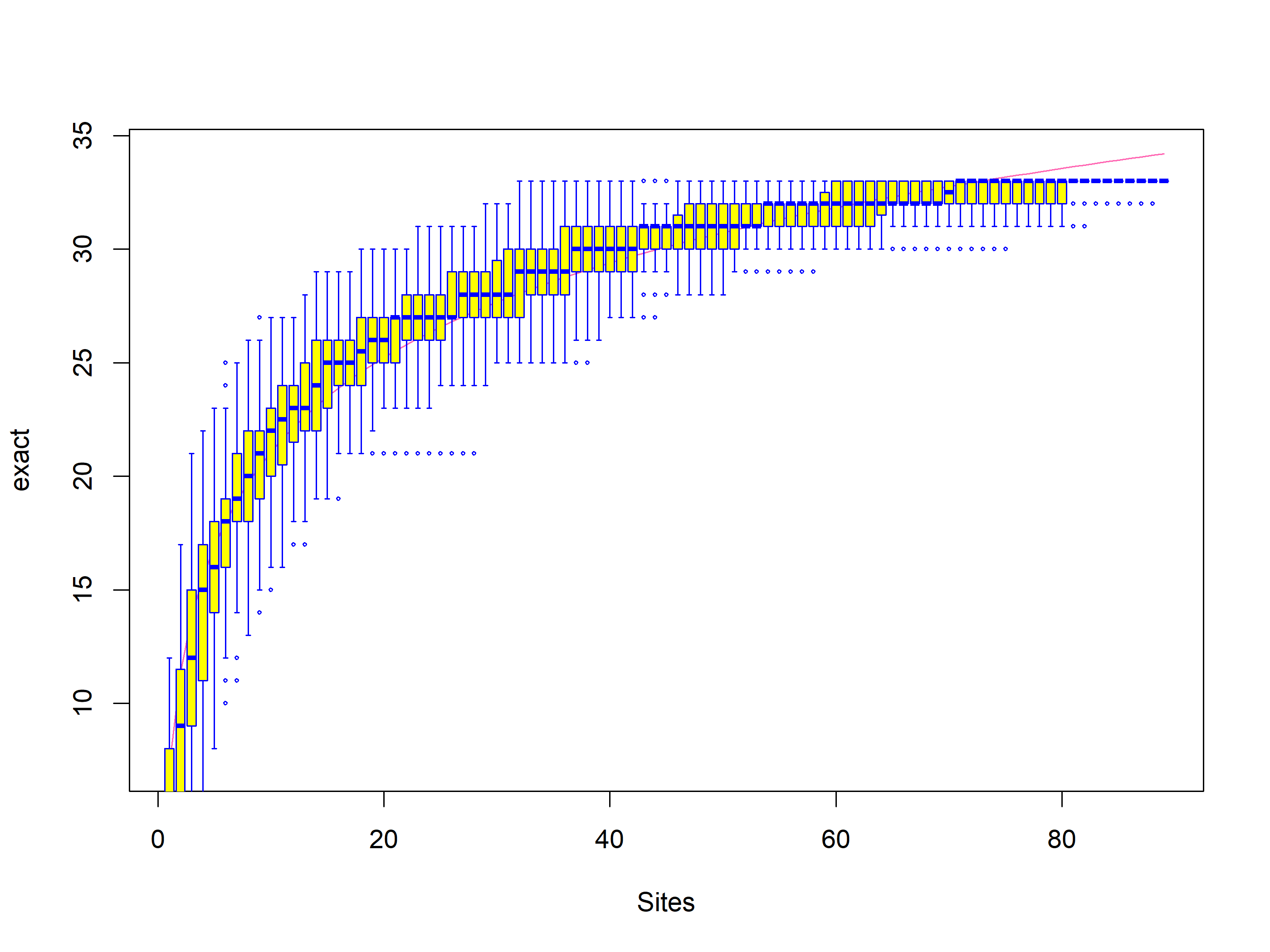
Species accumulation curves made using the package vegan, plot the increase in species richness as we add survey units. If the curve plateaus (flattens), then that suggests you have sampled the majority of the species in your survey site (camera or habitat type).
Code
# loop to make vegan matrixmat_vegan<-matrix(NA, dim(ylist[[1]])[1], length(unique(data_south$Species)))for(iin1:length(unique(data_south$Species))){mat_vegan[,i]<-apply(ylist[[i]], 1, sum, na.rm=TRUE)mat_vegan[,i]<-tidyr::replace_na(mat_vegan[,i], 0)# replace na with 0}colnames(mat_vegan)<-unique(data_south$Species)rownames(mat_vegan)<-rownames(ylist[[1]])mat_vegan2<-as.data.frame(mat_vegan)mat_vegan2$hab<-habs$hab_code# mat_vegan3 <- mat_vegan2 |> # Select specific rows by row numbersclosed_forest_rows<-which(mat_vegan2$hab=="closed_forest_evergreen_broad")herbaceous_rows<-which(mat_vegan2$hab=="herbaceous_wetland")herbs_rows<-which(mat_vegan2$hab=="herbs")open_forest_rows<-which(mat_vegan2$hab=="open_forest_evergreen_broad")open_forest2_rows<-which(mat_vegan2$hab=="open_forest_other")closed_forest<-apply(mat_vegan2[closed_forest_rows,1:22], MARGIN =2, sum)herbaceous_wetland<-apply(mat_vegan2[herbaceous_rows,1:22], MARGIN =2, sum)herbs<-apply(mat_vegan2[herbs_rows,1:22], MARGIN =2, sum)open_forest_evergreen<-apply(mat_vegan2[open_forest_rows,1:22], MARGIN =2, sum)open_forest_other<-apply(mat_vegan2[open_forest2_rows,1:22], MARGIN =2, sum)# tb_sp <- mat_vegan2 |> group_by(hab)# hab_list <- group_split(tb_sp)# make list of dataframe per habitatsp_by_hab<-mat_vegan2|>dplyr::group_by(hab)%>%split(.$hab)# arrange abundance (detection frecuency) mat for INEXT cesar_sp<-t(rbind(t(colSums(sp_by_hab[[1]][,1:33])),t(colSums(sp_by_hab[[2]][,1:33])),t(colSums(sp_by_hab[[3]][,1:33])),t(colSums(sp_by_hab[[4]][,1:33])),t(colSums(sp_by_hab[[5]][,1:33]))))colnames(cesar_sp)<-names(sp_by_hab)# function to Format data to incidence and use iNextf_incidences<-function(habitat_rows=closed_forest_rows){ylist%>%# historias de detectionmap(~rowSums(.,na.rm =T))%>%# sumo las detecciones en cada sitioreduce(cbind)%>%# unimos las listasas_data_frame()%>%#formato dataframefilter(row_number()%in%habitat_rows)|>t()%>%# trasponer la tablaas_tibble()%>%#formato tibblemutate_if(is.numeric,~(.>=1)*1)%>%#como es incidencia, formateo a 1 y 0rowSums()%>%# ahora si la suma de las incidencias en cada sitiosort(decreasing=T)|>as_tibble()%>%add_row(value=length(habitat_rows), .before =1)%>%# requiere que el primer valor sea el número de sitiosfilter(!if_any()==0)|># filter cerosas.matrix()# Requiere formato de matriz}# Make incidence frequency table (is a list whit 5 habitats)# Make an empty list to store our dataincidence_cesar<-list()incidence_cesar[[1]]<-f_incidences(closed_forest_rows)incidence_cesar[[2]]<-f_incidences(herbaceous_rows)incidence_cesar[[3]]<-f_incidences(herbs_rows)incidence_cesar[[4]]<-f_incidences(open_forest_rows)incidence_cesar[[5]]<-f_incidences(open_forest_other)# put namesnames(incidence_cesar)<-names(sp_by_hab)# we deleted this habitat type for making errorincidence_cesar<-within(incidence_cesar, rm("herbaceous_wetland"))
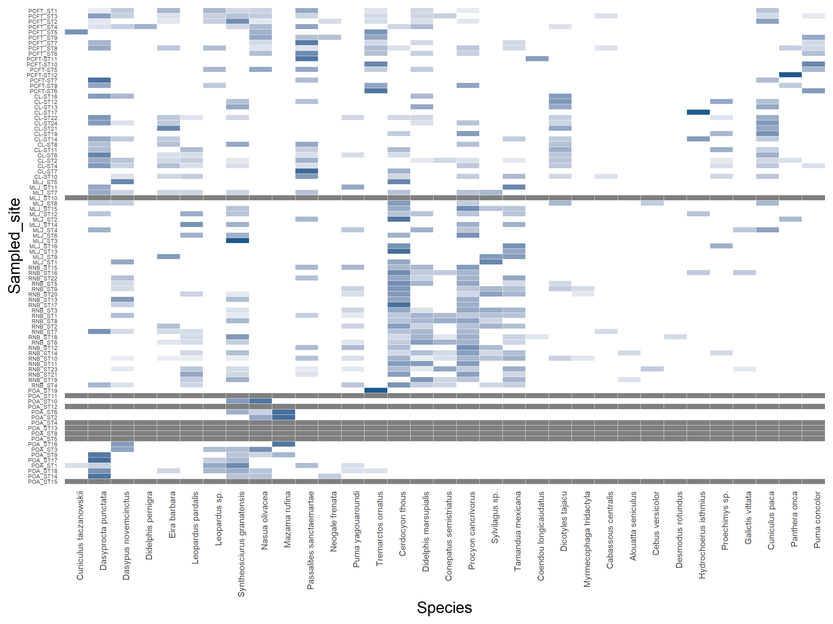
To start lets plot the species vs sites
Code
# Transpose if needed to have sample site names on rowsabund_table<-mat_vegan# Convert to relative frequenciesabund_table<-abund_table/rowSums(abund_table)library(reshape2)df<-melt(abund_table)colnames(df)<-c("Sampled_site","Species","Value")library(plyr)library(scales)# We are going to apply transformation to our data to make it# easier on eyes #df<-ddply(df,.(Samples),transform,rescale=scale(Value))df<-ddply(df,.(Sampled_site),transform,rescale=sqrt(Value))# Plot heatmapp<-ggplot(df, aes(Species, Sampled_site))+geom_tile(aes(fill =rescale),colour ="white")+scale_fill_gradient(low ="white",high ="#1E5A8C")+scale_x_discrete(expand =c(0, 0))+scale_y_discrete(expand =c(0, 0))+theme(legend.position ="none",axis.ticks =element_blank(),axis.text.x =element_text(angle =90, hjust =1,size=6),axis.text.y =element_text(size=4))# ggplotly(p) # see interactive# View the plotp
Notice how some cameras didn’t record any species. Here showed as the gay horizontal line. Perhaps we need to delete those cameras.
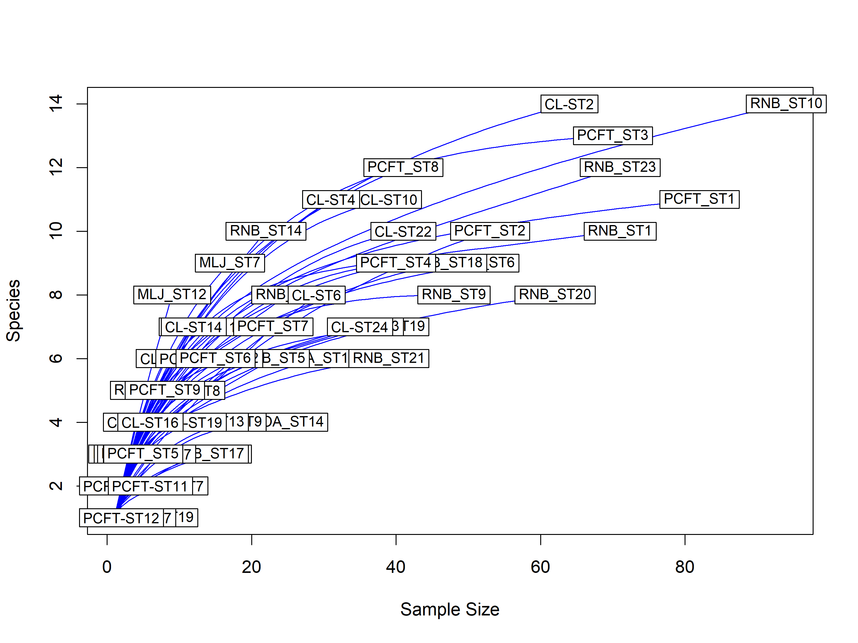
Rarefaction using vegan
Notice that sites are cameras and the accumulation is species per camera not time
Rarefaction is a technique to assess expected species richness. Rarefaction allows the calculation of species richness for a given number of individual samples, based on the construction of rarefaction curves.
The issue that occurs when sampling various species in a community is that the larger the number of individuals sampled, the more species that will be found. Rarefaction curves are created by randomly re-sampling the pool of N samples multiple times and then plotting the average number of species found in each sample (1,2, … N). “Thus rarefaction generates the expected number of species in a small collection of n individuals (or n samples) drawn at random from the large pool of N samples.”. Rarefaction curves generally grow rapidly at first, as the most common species are found, but the curves plateau as only the rarest species remain to be sampled.
In this step we convert the Cameratrap-operation table to sf, we add elevation from Amazon web Services (AWS), habitat type and species per site (S.chao1) to finally visualize the map showing the number of species as the size of the dot.
Code
# datos_distinct <- datos |> distinct(Longitude, Latitude, CT, Proyecto)projlatlon<-"+proj=longlat +datum=WGS84 +no_defs +ellps=WGS84 +towgs84=0,0,0"CToperation_sf<-st_as_sf(x =CToperation, coords =c("Longitude", "Latitude"), crs =projlatlon)# write.csv(habs, "C:/CodigoR/CameraTrapCesar/data/habitats.csv")habs<-read.csv("C:/CodigoR/CameraTrapCesar/data/habitats.csv")CToperation_elev_sf<-get_elev_point(CToperation_sf, src ="aws")# get elevation from AWSCToperation_elev_sf<-CToperation_elev_sf|>left_join(habs, by='Station')|>left_join(S_per_site, by='Station')|>select("Station", "elevation", "minStart.x","maxEnd.x", "Year.x", "hab_code" , "S.obs", "S.chao1")# add habitat # CToperation_elev_sf$habs <- habs$hab_code# see the mapmapview(CToperation_elev_sf, zcol="hab_code", cex ="S.chao1", alpha =0)
Perhaps it is easyer to plot the species number as a countour map
One advantage of using the eks density estimate, is that it is clearer what the output means. The 20% contour means “20% of the measurements lie inside this contour”. The documentation for eks takes issue with how stat_density_2d from ggplot2 does its calculation, I don’t know who is right because the estimated value is species and both graphs are similar.
Code
# select chaospecies<-dplyr::select(CToperation_elev_sf, "S.chao1")# hakeoides_coord <- data.frame(sf::st_coordinates(hakeoides))Sta_den<-eks::st_kde(species)# calculate density# VERY conveniently, eks can generate an sf file of contour linescontours<-eks::st_get_contour(Sta_den, cont=c(10,20,30,40,50,60,70,80, 90))%>%mutate(value=as.numeric(levels(contlabel)))# pal_fun <- leaflet::colorQuantile("YlOrRd", NULL, n = 5)p_popup<-paste("Species", as.numeric(levels(contours$estimate)), "number")tmap::tmap_mode("view")# set mode to interactive plotstmap::tm_shape(species)+tmap::tm_sf(col="black", size=0.2)+# contours from ekstmap::tm_shape(contours)+tmap::tm_polygons("estimate", palette="Reds", alpha=0.5)
In general terms the species estimate per site seems to be larger near the coal mine and decrease with the distance to the mine. Also notice kernel density estimates are larger than s.chao1.
Nonmetric Multidimensional Scaling (NMDS)
Often in ecological research, we are interested not only in comparing univariate descriptors of communities, like diversity, but also in how the constituent species — or the species composition — changes from one community to the next. One common tool to do this is non-metric multidimensional scaling, or NMDS. The goal of NMDS is to collapse information from multiple dimensions (e.g, from multiple communities, sites were the cameratrap was installed, etc.) into just a few, so that they can be visualized and interpreted. Unlike other ordination techniques that rely on (primarily Euclidean) distances, such as Principal Coordinates Analysis, NMDS uses rank orders, and thus is an extremely flexible technique that can accommodate a variety of different kinds of data.
If the treatment is continuous, such as an environmental gradient, then it might be useful to plot contour lines rather than convex hulls. We can get some, elevation data for our original community matrix and overlay them onto the NMDS plot using ordisurf.
Code
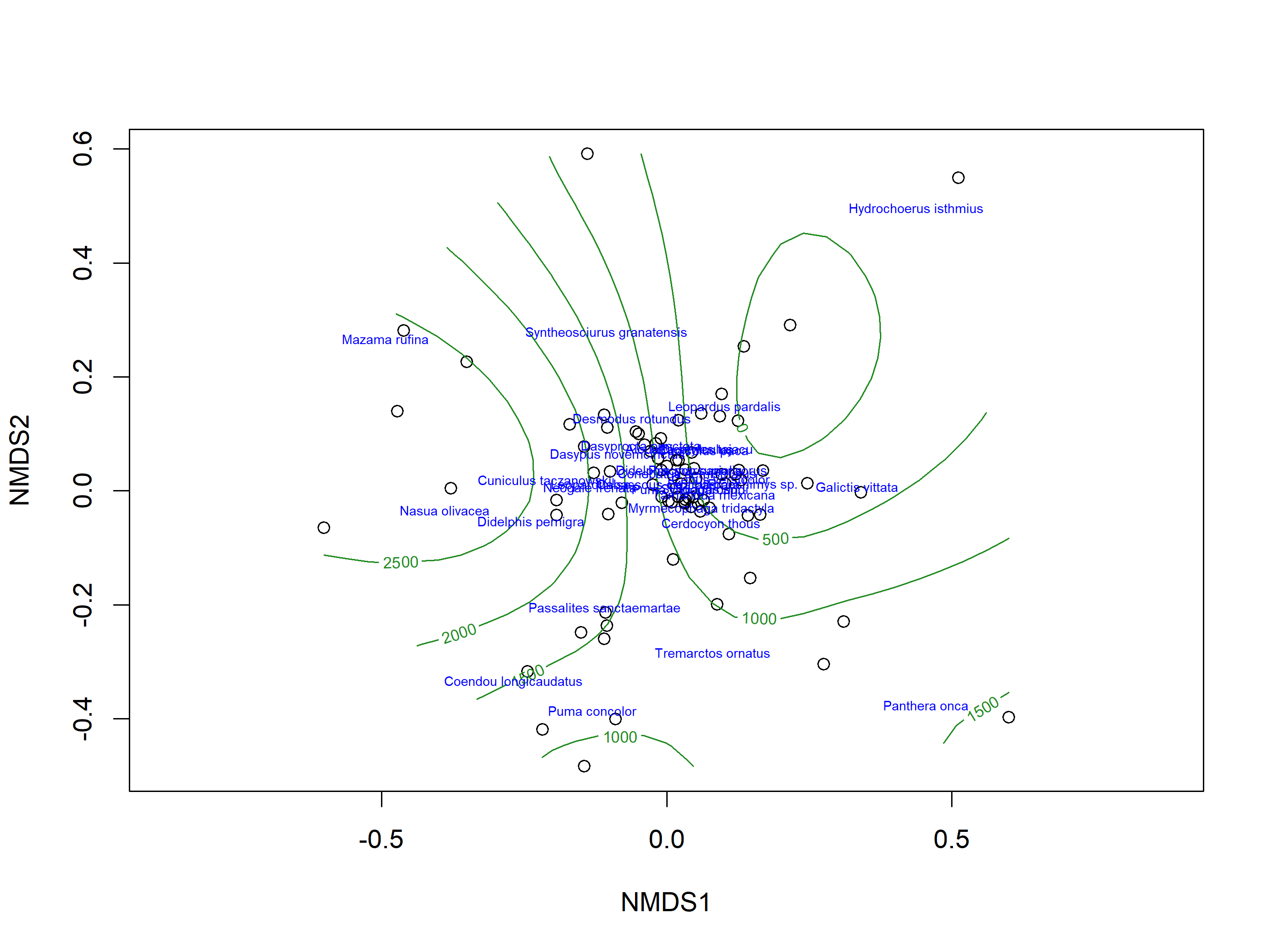
example_NMDS=metaMDS(as.data.frame(mat_vegan), distance="euclidean", zerodist ="ignore", trymax=300, k=5)# T#> Wisconsin double standardization#> Run 0 stress 0.1177774 #> Run 1 stress 0.1206288 #> Run 2 stress 0.1186686 #> Run 3 stress 0.1191797 #> Run 4 stress 0.1179719 #> ... Procrustes: rmse 0.05919246 max resid 0.2038165 #> Run 5 stress 0.1183849 #> Run 6 stress 0.1196809 #> Run 7 stress 0.1186472 #> Run 8 stress 0.1184403 #> Run 9 stress 0.1196989 #> Run 10 stress 0.1194615 #> Run 11 stress 0.1214856 #> Run 12 stress 0.1188458 #> Run 13 stress 0.1204449 #> Run 14 stress 0.1193109 #> Run 15 stress 0.118481 #> Run 16 stress 0.1195796 #> Run 17 stress 0.1186381 #> Run 18 stress 0.1191817 #> Run 19 stress 0.1176268 #> ... New best solution#> ... Procrustes: rmse 0.06730393 max resid 0.1981391 #> Run 20 stress 0.1188219 #> Run 21 stress 0.1185899 #> Run 22 stress 0.1203331 #> Run 23 stress 0.1194288 #> Run 24 stress 0.1201856 #> Run 25 stress 0.1202617 #> Run 26 stress 0.1181575 #> Run 27 stress 0.1202947 #> Run 28 stress 0.118683 #> Run 29 stress 0.119821 #> Run 30 stress 0.1194675 #> Run 31 stress 0.1210007 #> Run 32 stress 0.1184738 #> Run 33 stress 0.1195521 #> Run 34 stress 0.1187497 #> Run 35 stress 0.1191322 #> Run 36 stress 0.1179864 #> ... Procrustes: rmse 0.06264792 max resid 0.2506916 #> Run 37 stress 0.1185073 #> Run 38 stress 0.1192425 #> Run 39 stress 0.1187494 #> Run 40 stress 0.1178776 #> ... Procrustes: rmse 0.06673682 max resid 0.3230683 #> Run 41 stress 0.1191402 #> Run 42 stress 0.1183157 #> Run 43 stress 0.118886 #> Run 44 stress 0.118375 #> Run 45 stress 0.1210902 #> Run 46 stress 0.1183168 #> Run 47 stress 0.1200819 #> Run 48 stress 0.1188811 #> Run 49 stress 0.1190618 #> Run 50 stress 0.1190239 #> Run 51 stress 0.1192832 #> Run 52 stress 0.1171768 #> ... New best solution#> ... Procrustes: rmse 0.06292082 max resid 0.295684 #> Run 53 stress 0.1187272 #> Run 54 stress 0.1191086 #> Run 55 stress 0.1192896 #> Run 56 stress 0.1205005 #> Run 57 stress 0.1187612 #> Run 58 stress 0.119228 #> Run 59 stress 0.1190356 #> Run 60 stress 0.1179332 #> Run 61 stress 0.1197881 #> Run 62 stress 0.1181237 #> Run 63 stress 0.1193814 #> Run 64 stress 0.118903 #> Run 65 stress 0.1191659 #> Run 66 stress 0.1189552 #> Run 67 stress 0.118381 #> Run 68 stress 0.1182353 #> Run 69 stress 0.1185069 #> Run 70 stress 0.119889 #> Run 71 stress 0.1189324 #> Run 72 stress 0.1202498 #> Run 73 stress 0.1198287 #> Run 74 stress 0.1173791 #> ... Procrustes: rmse 0.03459135 max resid 0.1320568 #> Run 75 stress 0.118462 #> Run 76 stress 0.1208487 #> Run 77 stress 0.1184617 #> Run 78 stress 0.11866 #> Run 79 stress 0.1205182 #> Run 80 stress 0.1196904 #> Run 81 stress 0.1190856 #> Run 82 stress 0.1181391 #> Run 83 stress 0.1194442 #> Run 84 stress 0.1185924 #> Run 85 stress 0.1193937 #> Run 86 stress 0.121223 #> Run 87 stress 0.1180475 #> Run 88 stress 0.1172267 #> ... Procrustes: rmse 0.03409711 max resid 0.1753628 #> Run 89 stress 0.1192943 #> Run 90 stress 0.1196633 #> Run 91 stress 0.1188599 #> Run 92 stress 0.1183631 #> Run 93 stress 0.1187598 #> Run 94 stress 0.1185968 #> Run 95 stress 0.11951 #> Run 96 stress 0.1213391 #> Run 97 stress 0.1197127 #> Run 98 stress 0.119473 #> Run 99 stress 0.1196205 #> Run 100 stress 0.1192707 #> Run 101 stress 0.1187672 #> Run 102 stress 0.1193891 #> Run 103 stress 0.1180284 #> Run 104 stress 0.1203894 #> Run 105 stress 0.1194927 #> Run 106 stress 0.1212493 #> Run 107 stress 0.1182965 #> Run 108 stress 0.1202082 #> Run 109 stress 0.1196737 #> Run 110 stress 0.1184745 #> Run 111 stress 0.1196734 #> Run 112 stress 0.1210192 #> Run 113 stress 0.1204562 #> Run 114 stress 0.1183794 #> Run 115 stress 0.1196312 #> Run 116 stress 0.1195102 #> Run 117 stress 0.1186427 #> Run 118 stress 0.1177037 #> Run 119 stress 0.1196211 #> Run 120 stress 0.1184335 #> Run 121 stress 0.1187205 #> Run 122 stress 0.1193329 #> Run 123 stress 0.1183935 #> Run 124 stress 0.1180111 #> Run 125 stress 0.1190067 #> Run 126 stress 0.1199412 #> Run 127 stress 0.1203917 #> Run 128 stress 0.1193066 #> Run 129 stress 0.1190813 #> Run 130 stress 0.1210336 #> Run 131 stress 0.1183395 #> Run 132 stress 0.1185109 #> Run 133 stress 0.1186184 #> Run 134 stress 0.1182459 #> Run 135 stress 0.1190389 #> Run 136 stress 0.1204167 #> Run 137 stress 0.1186198 #> Run 138 stress 0.118966 #> Run 139 stress 0.1201539 #> Run 140 stress 0.1192333 #> Run 141 stress 0.1191073 #> Run 142 stress 0.1181058 #> Run 143 stress 0.1180379 #> Run 144 stress 0.1194509 #> Run 145 stress 0.1190307 #> Run 146 stress 0.1227532 #> Run 147 stress 0.1197243 #> Run 148 stress 0.1194925 #> Run 149 stress 0.1176478 #> ... Procrustes: rmse 0.03324642 max resid 0.1376792 #> Run 150 stress 0.1197673 #> Run 151 stress 0.118505 #> Run 152 stress 0.1195788 #> Run 153 stress 0.1183746 #> Run 154 stress 0.1207917 #> Run 155 stress 0.1195209 #> Run 156 stress 0.1186476 #> Run 157 stress 0.1205683 #> Run 158 stress 0.1203957 #> Run 159 stress 0.1194334 #> Run 160 stress 0.1187067 #> Run 161 stress 0.1191248 #> Run 162 stress 0.1194916 #> Run 163 stress 0.1187049 #> Run 164 stress 0.1188084 #> Run 165 stress 0.1195733 #> Run 166 stress 0.1189146 #> Run 167 stress 0.1189353 #> Run 168 stress 0.1190702 #> Run 169 stress 0.1188005 #> Run 170 stress 0.1188069 #> Run 171 stress 0.1199909 #> Run 172 stress 0.1198793 #> Run 173 stress 0.1193492 #> Run 174 stress 0.1183103 #> Run 175 stress 0.1188022 #> Run 176 stress 0.119465 #> Run 177 stress 0.1201642 #> Run 178 stress 0.1203076 #> Run 179 stress 0.1184545 #> Run 180 stress 0.1191182 #> Run 181 stress 0.1184663 #> Run 182 stress 0.1197293 #> Run 183 stress 0.1196431 #> Run 184 stress 0.1200847 #> Run 185 stress 0.1218445 #> Run 186 stress 0.1205694 #> Run 187 stress 0.1193901 #> Run 188 stress 0.1202695 #> Run 189 stress 0.1186335 #> Run 190 stress 0.1189535 #> Run 191 stress 0.1184268 #> Run 192 stress 0.1203722 #> Run 193 stress 0.11953 #> Run 194 stress 0.1181967 #> Run 195 stress 0.1210427 #> Run 196 stress 0.1193239 #> Run 197 stress 0.1189304 #> Run 198 stress 0.1188824 #> Run 199 stress 0.1179775 #> Run 200 stress 0.1200429 #> Run 201 stress 0.1186354 #> Run 202 stress 0.1175204 #> ... Procrustes: rmse 0.05732237 max resid 0.2698293 #> Run 203 stress 0.1190253 #> Run 204 stress 0.119378 #> Run 205 stress 0.1187723 #> Run 206 stress 0.1193228 #> Run 207 stress 0.1190969 #> Run 208 stress 0.1190627 #> Run 209 stress 0.1184325 #> Run 210 stress 0.1194397 #> Run 211 stress 0.1194828 #> Run 212 stress 0.1185745 #> Run 213 stress 0.1186796 #> Run 214 stress 0.1192906 #> Run 215 stress 0.1200002 #> Run 216 stress 0.1186742 #> Run 217 stress 0.119254 #> Run 218 stress 0.1191419 #> Run 219 stress 0.120306 #> Run 220 stress 0.119665 #> Run 221 stress 0.1212614 #> Run 222 stress 0.118446 #> Run 223 stress 0.1191734 #> Run 224 stress 0.1186459 #> Run 225 stress 0.1186136 #> Run 226 stress 0.1198339 #> Run 227 stress 0.1189743 #> Run 228 stress 0.1191247 #> Run 229 stress 0.1186571 #> Run 230 stress 0.1183342 #> Run 231 stress 0.120657 #> Run 232 stress 0.1200303 #> Run 233 stress 0.1194832 #> Run 234 stress 0.1183993 #> Run 235 stress 0.1192708 #> Run 236 stress 0.1195927 #> Run 237 stress 0.1192793 #> Run 238 stress 0.1203671 #> Run 239 stress 0.1187571 #> Run 240 stress 0.1206314 #> Run 241 stress 0.1172878 #> ... Procrustes: rmse 0.03546175 max resid 0.1313024 #> Run 242 stress 0.1180823 #> Run 243 stress 0.1204901 #> Run 244 stress 0.1190983 #> Run 245 stress 0.1199391 #> Run 246 stress 0.1182834 #> Run 247 stress 0.1184138 #> Run 248 stress 0.1205916 #> Run 249 stress 0.1173884 #> ... Procrustes: rmse 0.06476341 max resid 0.2793467 #> Run 250 stress 0.1184572 #> Run 251 stress 0.1179883 #> Run 252 stress 0.119103 #> Run 253 stress 0.1208135 #> Run 254 stress 0.1192279 #> Run 255 stress 0.1194243 #> Run 256 stress 0.1203805 #> Run 257 stress 0.1196346 #> Run 258 stress 0.1187809 #> Run 259 stress 0.1220039 #> Run 260 stress 0.1202155 #> Run 261 stress 0.119038 #> Run 262 stress 0.1185969 #> Run 263 stress 0.1185206 #> Run 264 stress 0.1191264 #> Run 265 stress 0.1203919 #> Run 266 stress 0.1193328 #> Run 267 stress 0.119689 #> Run 268 stress 0.1185788 #> Run 269 stress 0.1190655 #> Run 270 stress 0.1193243 #> Run 271 stress 0.1204081 #> Run 272 stress 0.1193853 #> Run 273 stress 0.1191507 #> Run 274 stress 0.1191006 #> Run 275 stress 0.1194524 #> Run 276 stress 0.1196515 #> Run 277 stress 0.1191174 #> Run 278 stress 0.1197212 #> Run 279 stress 0.1195057 #> Run 280 stress 0.1190863 #> Run 281 stress 0.1173829 #> ... Procrustes: rmse 0.04228723 max resid 0.2906148 #> Run 282 stress 0.1183771 #> Run 283 stress 0.118756 #> Run 284 stress 0.1184836 #> Run 285 stress 0.1193089 #> Run 286 stress 0.1187367 #> Run 287 stress 0.1211166 #> Run 288 stress 0.118612 #> Run 289 stress 0.1182366 #> Run 290 stress 0.1190942 #> Run 291 stress 0.118254 #> Run 292 stress 0.1182043 #> Run 293 stress 0.1210657 #> Run 294 stress 0.1176667 #> ... Procrustes: rmse 0.0316457 max resid 0.1553559 #> Run 295 stress 0.1180872 #> Run 296 stress 0.1173496 #> ... Procrustes: rmse 0.05887519 max resid 0.229526 #> Run 297 stress 0.1178518 #> Run 298 stress 0.1220267 #> Run 299 stress 0.1186454 #> Run 300 stress 0.1205719 #> *** Best solution was not repeated -- monoMDS stopping criteria:#> 300: no. of iterations >= maxit# plot the graphvegan::ordisurf((example_NMDS),CToperation_elev_sf$elevation,main="",col="forestgreen", trymax=100)# bubble = 2#> #> Family: gaussian #> Link function: identity #> #> Formula:#> y ~ s(x1, x2, k = 10, bs = "tp", fx = FALSE)#> #> Estimated degrees of freedom:#> 5.1 total = 6.1 #> #> REML score: 732.1451vegan::orditorp(example_NMDS,display="species",col="blue",air=0.1, cex=0.5)
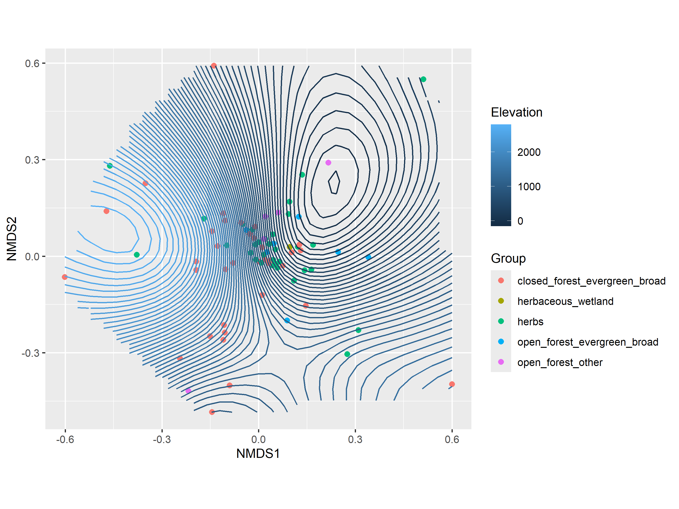
We can make a similar plot using gg_ordisurf from the package ggordiplots but also incorporating habitat type.
Code
# ggordiplots::gg_ordisurf()# To fit a surface with ggordiplots:ordiplot<-gg_ordisurf(ord =example_NMDS, env.var =CToperation_elev_sf$elevation, var.label ="Elevation", pt.size =2, groups =CToperation_elev_sf$hab_code, binwidth =50)
The contours connect species in the ordination space that are predicted to have the same elevation. Notice this is not a geographic map, it is a multivariate space.
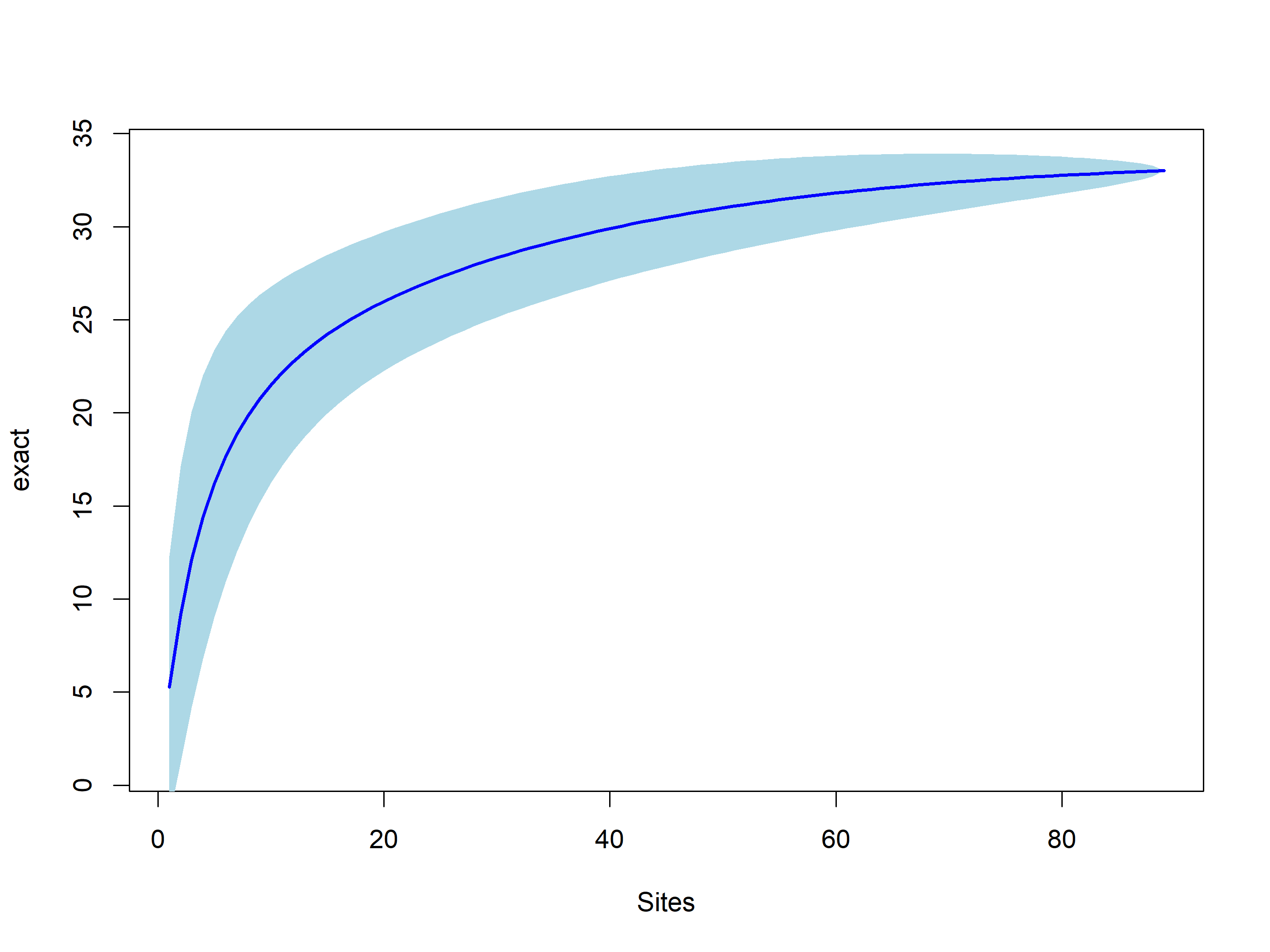
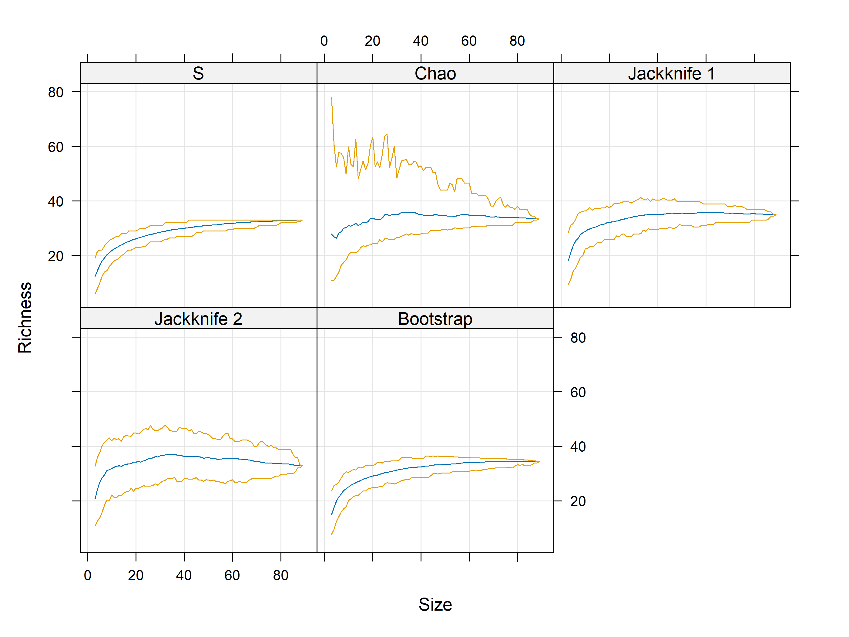
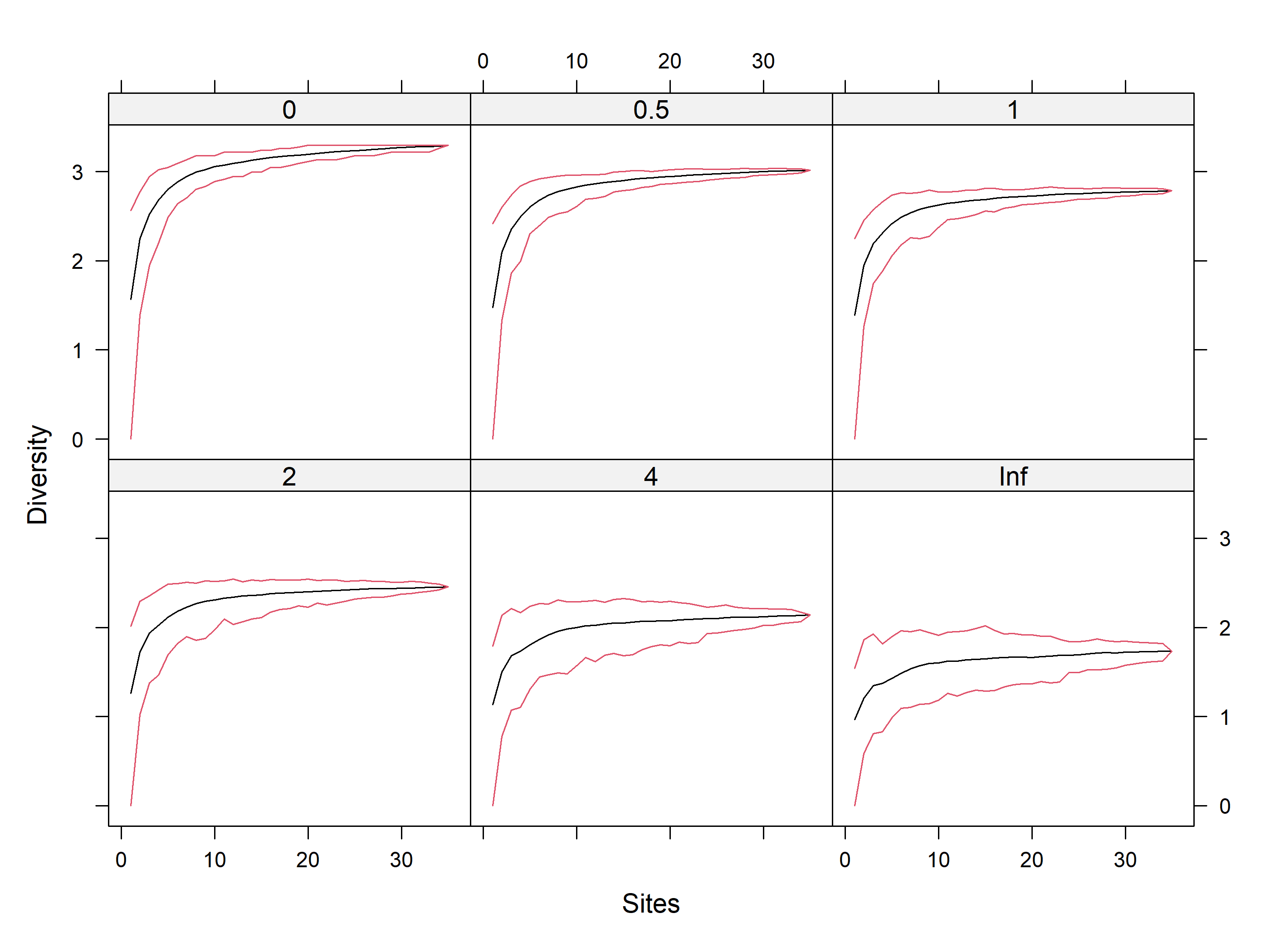
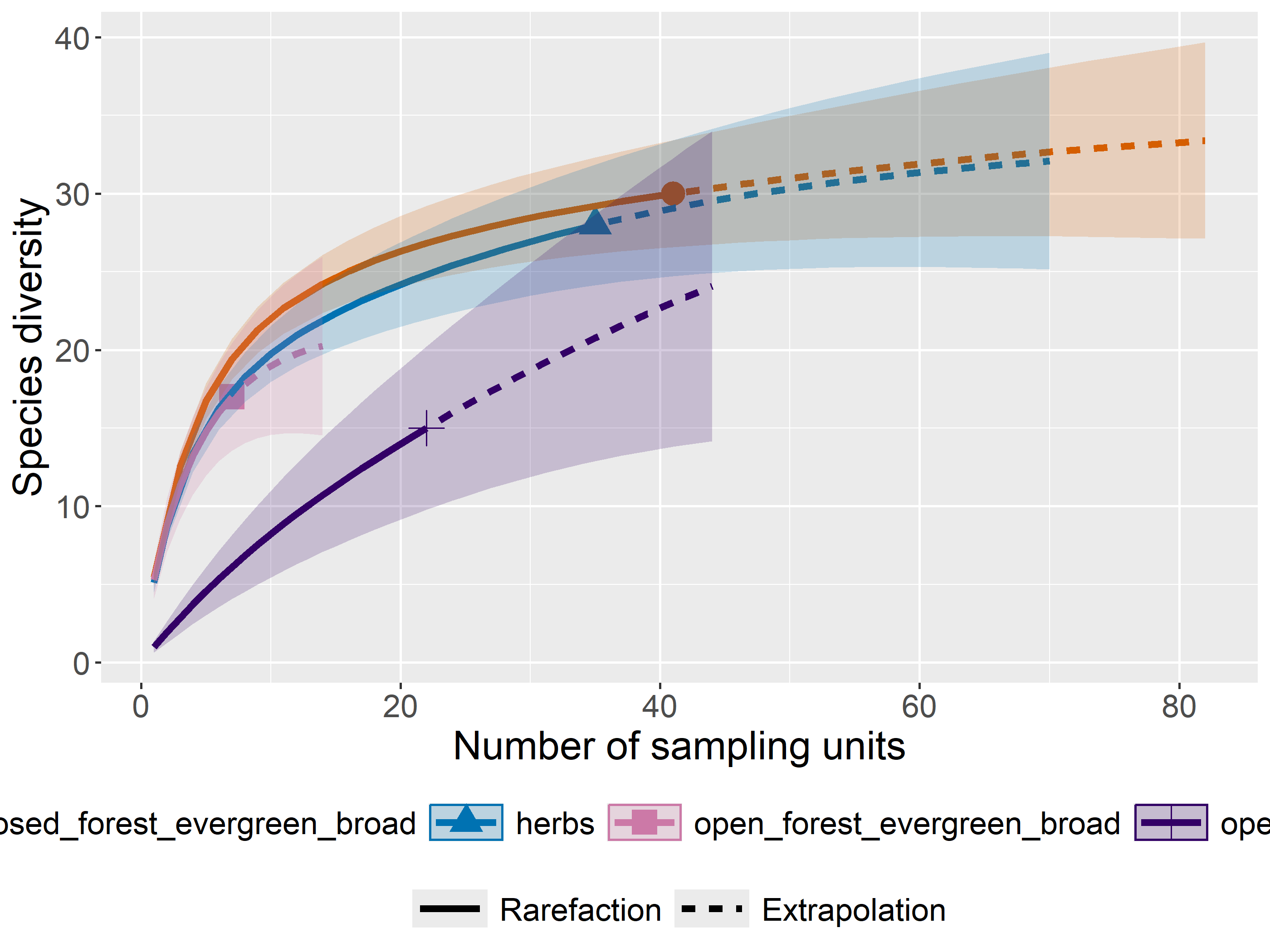
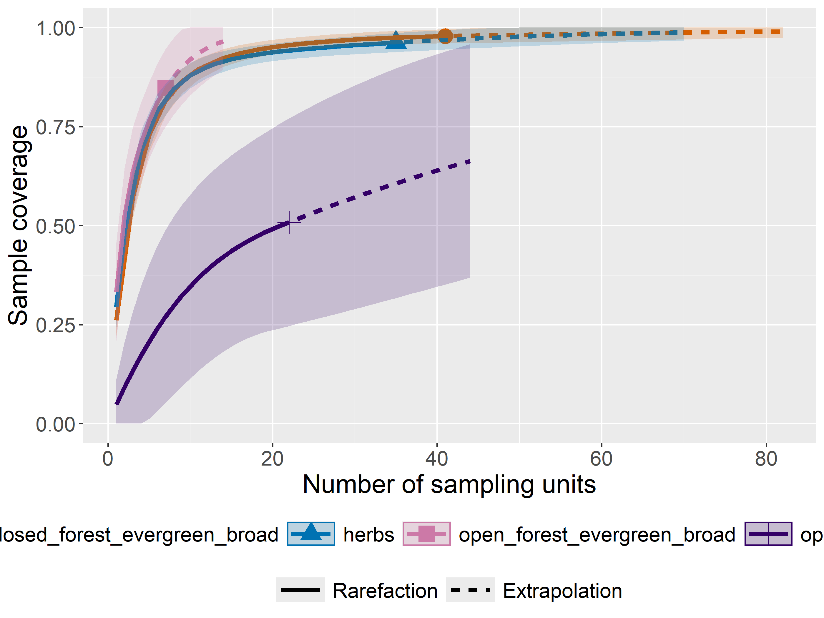
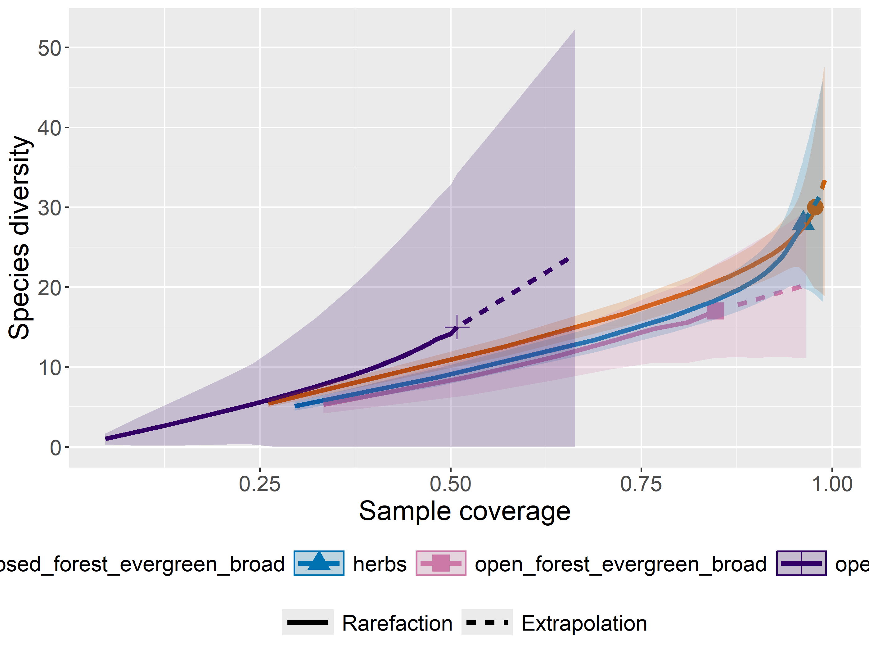
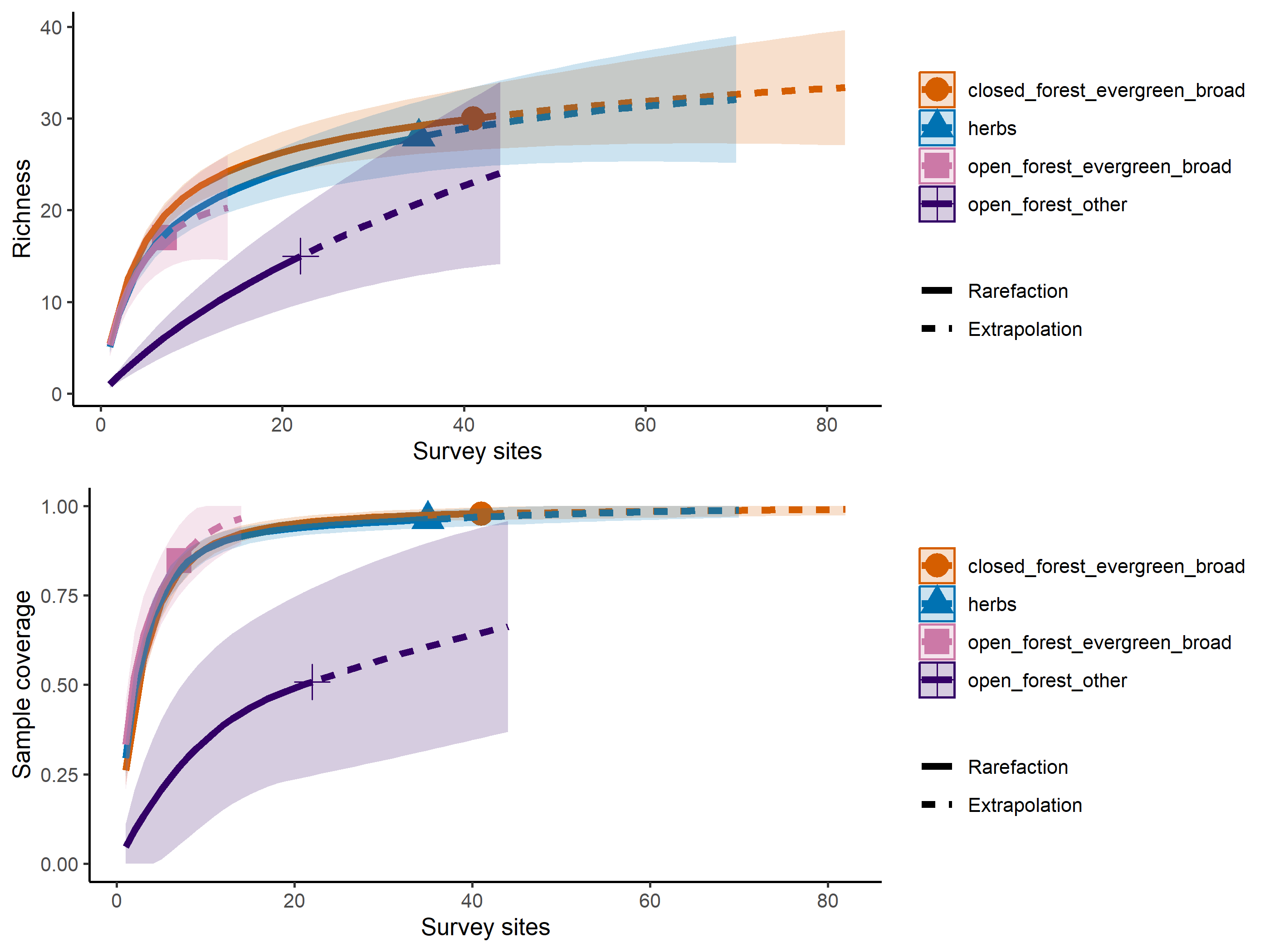
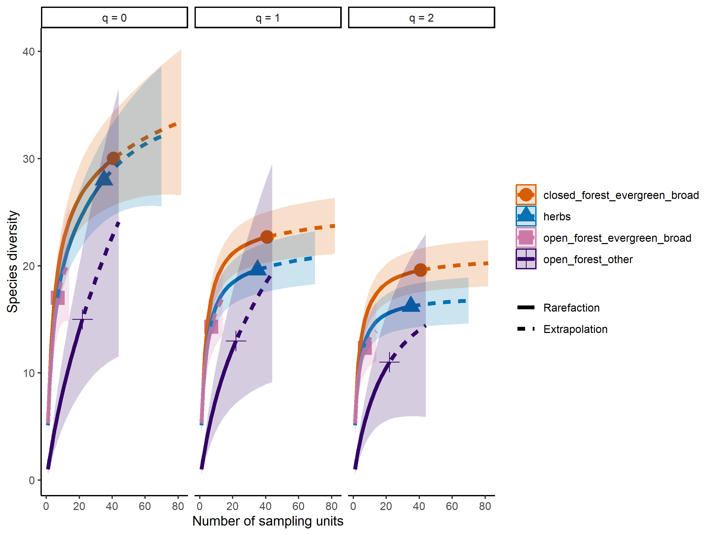
Rarefaction using iNEXT
Code
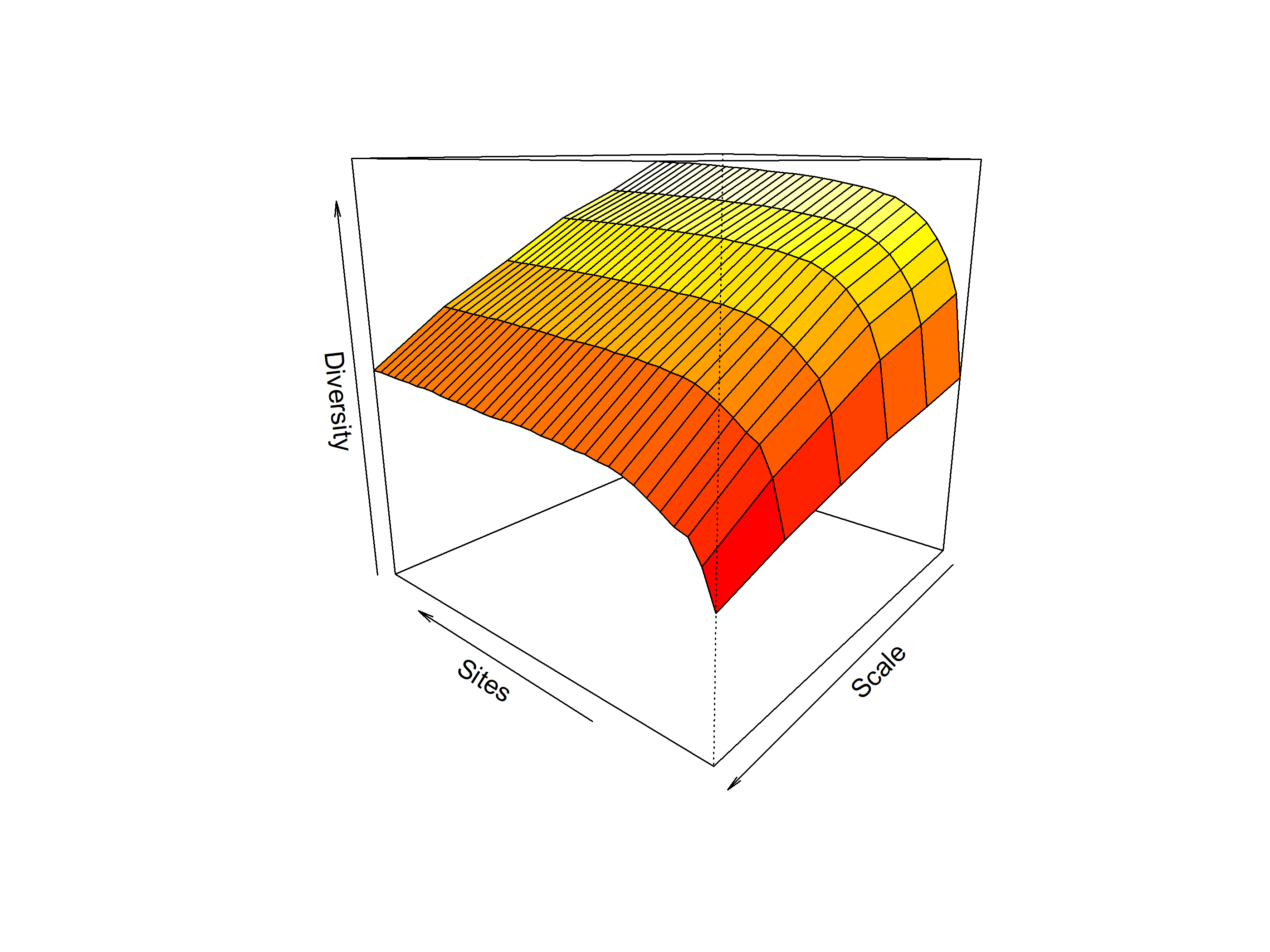
out<-iNEXT(incidence_cesar, # The data frame q=0,# The type of diversity estimator datatype="incidence_freq", # The type of analysis knots=40, # The number of data points se=TRUE, # confidence intervals conf=0.95, # The level of confidence intervals nboot=100)# The number of bootstraps ggiNEXT(out, type=1)
The iNEXT package is well suited for comparisons of diversity indices through the use of hill numbers - of which the q value = 1 represents the traditional diversity indices: The species richness is q = 0. The Shannon index is (q=1), and Simpson is (q=2). Note Increasing values of q reduces the influence of rare species on our estimate of community diversity.
Appelhans, Tim, Florian Detsch, Christoph Reudenbach, and Stefan Woellauer. 2025. mapview: Interactive Viewing of Spatial Data in r. https://CRAN.R-project.org/package=mapview.
Chao, Anne, Nicholas J. Gotelli, T. C. Hsieh, et al. 2014. “Rarefaction and Extrapolation with Hill Numbers: A Framework for Sampling and Estimation in Species Diversity Studies.”Ecological Monographs 84: 45–67.
Chao, Anne, K. H. Ma, T. C. Hsieh, and Chun-Huo Chiu. 2016. SpadeR: Species-Richness Prediction and Diversity Estimation with r. https://CRAN.R-project.org/package=SpadeR.
Hollister, Jeffrey, Tarak Shah, Jakub Nowosad, Alec L. Robitaille, Marcus W. Beck, and Mike Johnson. 2023. elevatr: Access Elevation Data from Various APIs. https://doi.org/10.5281/zenodo.8335450.
Niedballa, Jürgen, Rahel Sollmann, Alexandre Courtiol, and Andreas Wilting. 2016. “camtrapR: An r Package for Efficient Camera Trap Data Management.”Methods in Ecology and Evolution 7 (12): 1457–62. https://doi.org/10.1111/2041-210X.12600.
Pebesma, Edzer. 2018. “Simple Features for R: Standardized Support for Spatial Vector Data.”The R Journal 10 (1): 439–46. https://doi.org/10.32614/RJ-2018-009.
Wickham, Hadley. 2007. “Reshaping Data with the reshape Package.”Journal of Statistical Software 21 (12): 1–20. http://www.jstatsoft.org/v21/i12/.
Wickham, Hadley. 2011. “The Split-Apply-Combine Strategy for Data Analysis.”Journal of Statistical Software 40 (1): 1–29. https://www.jstatsoft.org/v40/i01/.
Wickham, Hadley, Mara Averick, Jennifer Bryan, et al. 2019. “Welcome to the tidyverse.”Journal of Open Source Software 4 (43): 1686. https://doi.org/10.21105/joss.01686.
Xie, Yihui. 2014. “knitr: A Comprehensive Tool for Reproducible Research in R.” In Implementing Reproducible Computational Research, edited by Victoria Stodden, Friedrich Leisch, and Roger D. Peng. Chapman; Hall/CRC.
Xie, Yihui. 2015. Dynamic Documents with R and Knitr. 2nd ed. Chapman; Hall/CRC. https://yihui.org/knitr/.
Xie, Yihui. 2025. knitr: A General-Purpose Package for Dynamic Report Generation in R. https://yihui.org/knitr/.
Xie, Yihui, J. J. Allaire, and Garrett Grolemund. 2018. R Markdown: The Definitive Guide. Chapman; Hall/CRC. https://bookdown.org/yihui/rmarkdown.
Xie, Yihui, Joe Cheng, Xianying Tan, and Garrick Aden-Buie. 2025. DT: A Wrapper of the JavaScript Library “DataTables”. https://CRAN.R-project.org/package=DT.