“Stacked” Models – Camera Trap Blog

Using random effects with `ubms`

One of the advantages of ubms is that it is possible to include random effects in your models, using the same syntax as lme4 (Bates et al. 2015). For example, if you have a group site covariate, you can fit a model with random intercepts by group by including + (1|group) in your parameter formula. Random slopes, or a combination of random slopes and intercepts, are also possible.

To illustrate the use of random effects of ubms, in this post fits we fit a model using a “stacked” model approach. Additionally in ubms you can instead include, for example, random site intercepts to account for possible pseudoreplication.

The “stacked” model

An alternative approach is to fit multiple years of data into a single-season model is using the “stacked” approach. Essentially, you treat unique site-year combinations as sites.

There are several potential reasons for this:

1. You don’t have enough data. Take in to account, Dail-Madsen type models are particularly data hungry.
1. You are not interested in the transition probabilities.
1. You have very few years or seasons (less than five) and the occupancy did not changed.

Load packages

First we load some packages

Code


library(grateful) # Facilitate Citation of R Packages
library(patchwork) # The Composer of Plots
library(readxl) # Read Excel Files
library(sf) # Simple Features for R
library(mapview) # Interactive Viewing of Spatial Data in R
library(terra) # Spatial Data Analysis
library(elevatr) # Access Elevation Data from Various APIs
library(readr)

library(camtrapR) # Camera Trap Data Management and Preparation of Occupancy and Spatial Capture-Recapture Analyses 
library(ubms) 
library(lme4) 
library(DT)

library(kableExtra) # Construct Complex Table with 'kable' and Pipe Syntax
library(tidyverse) # Easily Install and Load the 'Tidyverse'

Load data

The data set is downloaded from Initiative Monitoreo Katios in Wildlife insights

Code


path <- "C:/CodigoR/CameraTrapCesar/data/katios/"
cameras <- read_csv(paste(path, "cameras.csv", sep=""))
deployment <- read_csv(paste(path, "deployments.csv", sep=""))
images <- read_csv(paste(path, "images.csv", sep=""))
project <- read_csv(paste(path, "projects.csv", sep=""))

# join_by(project_id, camera_id, camera_name)`
cam_deploy <- cameras |> left_join(deployment) |> 
  dplyr::mutate(year=lubridate::year(start_date)) #|> filter(year== 2023)
cam_deploy_image <- images  |> 
  left_join(cam_deploy) |> 
  mutate(scientificName= paste(genus, species, sep = " ")) |> 
   mutate(deployment_id_cam=paste(deployment_id, camera_id, sep = "-")) #|> 
  # filter(year==2022)

Convert to sf and view the map

Code


datos_distinct <- cam_deploy_image |> distinct(longitude, latitude, deployment_id, samp_year) |> as.data.frame()

# Fix NA camera 16
datos_distinct[16,] <- c( -77.2787, 7.73855, 
                      "CT-K1-31-124", 2021)

projlatlon <- "+proj=longlat +datum=WGS84 +no_defs +ellps=WGS84 +towgs84=0,0,0"

datos_sf <-  st_as_sf(x = datos_distinct,
                         coords = c("longitude", 
                                    "latitude"),
                         crs = projlatlon)

mapview(st_jitter(datos_sf, 0.00075) , zcol="samp_year")

Notice we used the function st_jitter() because the points are on top of the previous year.

Extract site covariates

Using the coordinates of the sf object (datos_sf) we put the cameras on top of the covaraies and with the function terra::extract() we get the covariate value.

In this case we used as covariates:

Cattle distribution as number of cows per 10 square kilometer (Gilbert et al. 2018).
Percent of tree cover from MODIS product 44B.
Road density from (Meijer et al. 2018).
Land cover types from MODIS.

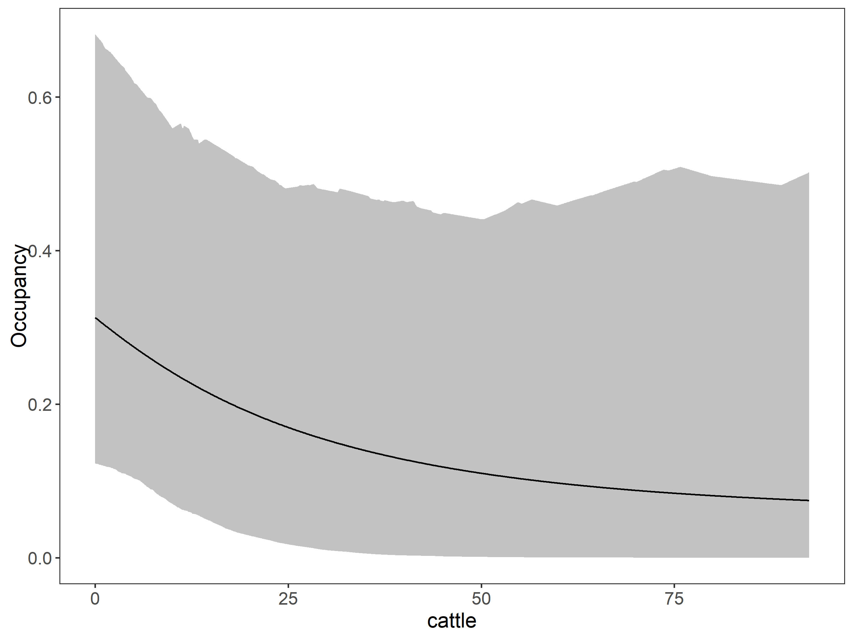
Code

#load rasters
per_tree_cov <- rast("C:/CodigoR/WCS-CameraTrap/raster/latlon/Veg_Cont_Fields_Yearly_250m_v61/Perc_TreeCov/MOD44B_Perc_TreeCov_2021_065.tif")
road_den <- rast("C:/CodigoR/WCS-CameraTrap/raster/latlon/RoadDensity/grip4_total_dens_m_km2.asc")
# elev <- rast("D:/CORREGIDAS/elevation_z7.tif")
landcov <- rast("C:/CodigoR/WCS-CameraTrap/raster/latlon/LandCover_Type_Yearly_500m_v61/LC1/MCD12Q1_LC1_2021_001.tif") 
cattle <- rast("C:/CodigoR/WCS-CameraTrap/raster/latlon/Global cattle distribution/5_Ct_2010_Da.tif")
#river <- st_read("F:/WCS-CameraTrap/shp/DensidadRios/MCD12Q1_LC1_2001_001_RECLASS_MASK_GRID_3600m_DensDrenSouthAmer.shp")

# get elevation map
# elevation_detailed <- rast(get_elev_raster(sites, z = 10, clip="bbox", neg_to_na=TRUE))
# elevation_detailed <- get_elev_point (datos_sf, src="aws", overwrite=TRUE)


# extract covs using points and add to sites
# covs <- cbind(sites, terra::extract(SiteCovsRast, sites))
per_tre <- terra::extract(per_tree_cov, datos_sf)
roads <- terra::extract(road_den, datos_sf)
# eleva <- terra::extract(elevation_detailed, sites)
land_cov <- terra::extract(landcov, datos_sf)
cattle_den <-  terra::extract(cattle, datos_sf)

#### drop geometry 
sites <- datos_sf %>%
  mutate(lat = st_coordinates(.)[,1],
         lon = st_coordinates(.)[,2]) %>%
  st_drop_geometry() |> as.data.frame()

# remove decimals convert to factor
sites$land_cover <-  factor(land_cov$MCD12Q1_LC1_2021_001)
# sites$elevation <-  eleva$file3be898018c3
sites$per_tree_cov <- per_tre$MOD44B_Perc_TreeCov_2021_065 
#  fix 200 isue
ind <- which(sites$per_tree_cov== 200)
sites$per_tree_cov[ind] <- 0

# sites$elevation <- elevation_detailed$elevation
sites$roads <- roads$grip4_total_dens_m_km2
sites$cattle <- cattle_den[,2]


write.csv(sites, "C:/CodigoR/CameraTrapCesar/data/katios/stacked/site_covs.csv")

Select by years and convert to stacked format

To get the detection history we use the function detectionHistory of the camtrapR package.

But take in to account, at the end we need to stack the data in this format:

obs1	obs2	obs3	site	year
0	0	0	1	1
0	0	0	2	1
NA	NA	NA	3	1
0	0	0	4	1
0	0	0	5	2
NA	NA	NA	6	2

So we need to go by years and then stack de two tables.

First year 2021

Here we use the function detectionHistory() to generate species detection histories that can be used in occupancy analyses, with package unmarked and ubms. It generates detection histories in different formats, with adjustable occasion length and occasion start time. Notice we firs neet to get the camera operation dates using the function cameraOperation().

Code


# filter first year and make uniques

CToperation_2021  <- cam_deploy_image |> #multi-season data
  filter(samp_year==2021) |> 
  group_by(deployment_id) |> 
  mutate(minStart=min(start_date), maxEnd=max(end_date)) |> 
  distinct(longitude, latitude, minStart, maxEnd, samp_year) |> 
  ungroup() |> as.data.frame()


# Fix NA camera 16
CToperation_2021[16,] <- c("CT-K1-31-124", -77.2787,    7.73855, 
                      "2021-10-10", "2021-12-31", 2021)

# make numeric sampling year
CToperation_2021$samp_year <- as.numeric(CToperation_2021$samp_year)

# camera operation matrix for _2021
# multi-season data. Season1
camop_2021 <- cameraOperation(CTtable= CToperation_2021, # Tabla de operación
                         stationCol= "deployment_id", # Columna que define la estación
                         setupCol= "minStart", #Columna fecha de colocación
                         retrievalCol= "maxEnd", #Columna fecha de retiro
                         sessionCol = "samp_year", # multi-season column
                         #hasProblems= T, # Hubo fallos de cámaras
                         dateFormat= "%Y-%m-%d")#, #, # Formato de las fechas
                         #cameraCol="CT")
                         #sessionCol= "samp_year")

# Generar las historias de detección ---------------------------------------
## remove plroblem species
# ind <- which(datos_PCF$Species=="Marmosa sp.")
# datos_PCF <- datos_PCF[-ind,]

# filter y1
datay_2021 <- cam_deploy_image |> filter(samp_year ==2021) # |> 
  # filter(samp_year==2022) 

DetHist_list_2021 <- lapply(unique(datay_2021$scientificName), FUN = function(x) {
  detectionHistory(
    recordTable         = datay_2021, # Tabla de registros
    camOp                = camop_2021, # Matriz de operación de cámaras
    stationCol           = "deployment_id",
    speciesCol           = "scientificName",
    recordDateTimeCol    = "timestamp",
    recordDateTimeFormat  = "%Y-%m-%d %H:%M:%S",
    species              = x,     # la función reemplaza x por cada una de las especies
    occasionLength       = 15, # Colapso de las historias a días
    day1                 = "station", #inicie en la fecha de cada survey
    datesAsOccasionNames = FALSE,
    includeEffort        = TRUE,
    scaleEffort          = FALSE,
    unmarkedMultFrameInput=TRUE,
    timeZone             = "America/Bogota" 
    )
  }
)

# names
names(DetHist_list_2021) <- unique(datay_2021$scientificName)

# Finalmente creamos una lista nueva donde estén solo las historias de detección
ylist_2021 <- lapply(DetHist_list_2021, FUN = function(x) x$detection_history)
# y el esfuerzo
effortlist_2021 <- lapply(DetHist_list_2021, FUN = function(x) x$effort)

### Danta, Jaguar
which(names(ylist_2021) =="Tapirus bairdii")
#> integer(0)
which(names(ylist_2021) =="Panthera onca") 
#> [1] 5

Next, the year 2022

Code


# filter firs year and make uniques

CToperation_2022  <- cam_deploy_image |> #multi-season data
  filter(samp_year==2022) |> 
  group_by(deployment_id) |> 
  mutate(minStart=min(start_date), maxEnd=max(end_date)) |> 
  distinct(longitude, latitude, minStart, maxEnd, samp_year) |> 
  ungroup() |> as.data.frame()


# Fix NA camera 16
# CToperation_2022[16,] <- c("CT-K1-31-124", -77.2787,  7.73855, 
#                       "2022-10-10", "2022-12-31", 2022)

# make numeric sampling year
CToperation_2022$samp_year <- as.numeric(CToperation_2022$samp_year)

# camera operation matrix for _2022
# multi-season data. Season1
camop_2022 <- cameraOperation(CTtable= CToperation_2022, # Tabla de operación
                         stationCol= "deployment_id", # Columna que define la estación
                         setupCol= "minStart", #Columna fecha de colocación
                         retrievalCol= "maxEnd", #Columna fecha de retiro
                         sessionCol = "samp_year", # multi-season column
                         #hasProblems= T, # Hubo fallos de cámaras
                         dateFormat= "%Y-%m-%d")#, #, # Formato de las fechas
                         #cameraCol="CT")
                         #sessionCol= "samp_year")

# Generar las historias de detección ---------------------------------------
## remove plroblem species
# ind <- which(datos_PCF$Species=="Marmosa sp.")
# datos_PCF <- datos_PCF[-ind,]

# filter y1
datay_2022 <- cam_deploy_image |> filter(samp_year ==2022) # |> 
  # filter(samp_year==2022) 

DetHist_list_2022 <- lapply(unique(datay_2022$scientificName), FUN = function(x) {
  detectionHistory(
    recordTable         = datay_2022, # Tabla de registros
    camOp                = camop_2022, # Matriz de operación de cámaras
    stationCol           = "deployment_id",
    speciesCol           = "scientificName",
    recordDateTimeCol    = "timestamp",
    recordDateTimeFormat  = "%Y-%m-%d %H:%M:%S",
    species              = x,     # la función reemplaza x por cada una de las especies
    occasionLength       = 25, # Colapso de las historias a días
    day1                 = "station", #inicie en la fecha de cada survey
    datesAsOccasionNames = FALSE,
    includeEffort        = TRUE,
    scaleEffort          = FALSE,
    unmarkedMultFrameInput=TRUE,
    timeZone             = "America/Bogota" 
    )
  }
)

# names
names(DetHist_list_2022) <- unique(datay_2022$scientificName)

# Finalmente creamos una lista nueva donde estén solo las historias de detección
ylist_2022 <- lapply(DetHist_list_2022, FUN = function(x) x$detection_history)
effortlist_2022 <- lapply(DetHist_list_2022, FUN = function(x) x$effort)

### Danta, Jaguar
### Danta, Jaguar
which(names(ylist_2022) =="Tapirus bairdii")
#> [1] 21
which(names(ylist_2022) =="Panthera onca") 
#> [1] 19

Save and fix in excel

Jaguar

Code

# Jaguar
# datatable (ylist_2021[[5]], caption = 'Jaguar 2021')
# datatable (ylist_2022[[19]], caption = 'Jaguar 2022')

# y obs
write.csv(ylist_2021[[5]], "C:/CodigoR/CameraTrapCesar/data/katios/stacked/y_jaguar2021.csv")
# effort
write.csv(effortlist_2021[[5]], "C:/CodigoR/CameraTrapCesar/data/katios/stacked/effort_jaguar2021.csv")
# y obs
write.csv(ylist_2022[[19]], "C:/CodigoR/CameraTrapCesar/data/katios/stacked/y_jaguar2022.csv")
# effort
write.csv(effortlist_2022[[5]], "C:/CodigoR/CameraTrapCesar/data/katios/stacked/effort_jaguar2022.csv")

Fitting a stacked model for jaguar

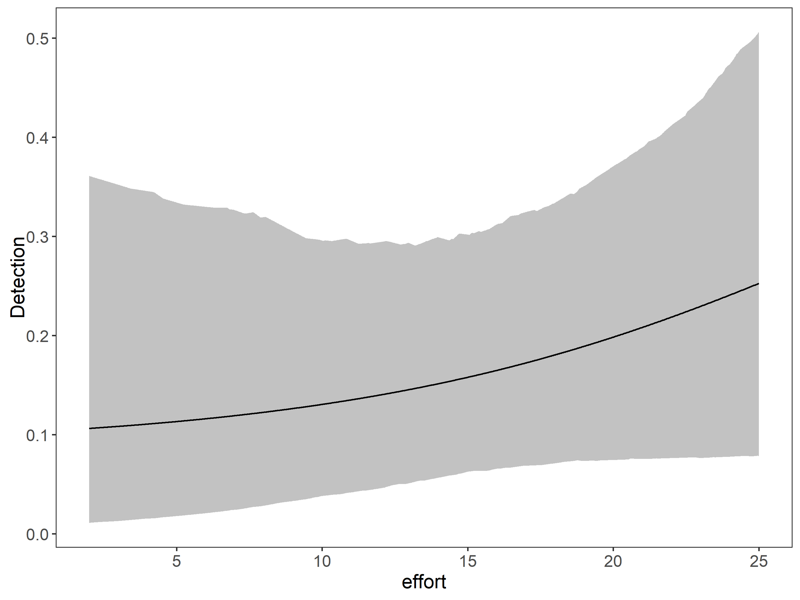
Lets use the ubms package to make a stacked occupancy model pooling 2021 and 2022 data together and use the percent tree cover, the road density and the cattle density as covariates for the occupancy and the effort as the number of sampling days as covariate for detection.

Load the data

Code

jaguar <- read.csv("C:/CodigoR/CameraTrapCesar/data/katios/stacked/y_jaguar_stacked.csv")

Look at the data

Code

datatable(head(jaguar))

Notice we collapsed the events to 15 days in the 2021 sampling season, and to 25 days in the 2022 sampling season, to end with 6 repeated observations in de matrix. In the matrix o1 to o6 are observations and e1 to e6 are sampling effort(observation covariates). Land_cover, per_tree_cov and roads are site covariates.

Create an unmarked frame

With our stacked dataset constructed, we build the unmarkedFrame() object.

Code


# fix NA spread
# yj <- rbind(ylist[[62]][1:30,1:8], # 62 is Jaguar
#             ylist[[62]][31:50,12:19])

# ej <- rbind(effortlist[[4]][1:30,1:8],
#             effortlist[[4]][31:50,12:19])
    
  
umf <- unmarkedFrameOccu(y=jaguar[,2:7], 
                         siteCovs=jaguar[,c(8,9,16:19)],
                         obsCovs=list(effort=jaguar[10:15])
                      )

plot(umf)

Fit models

Fit the Stacked Model

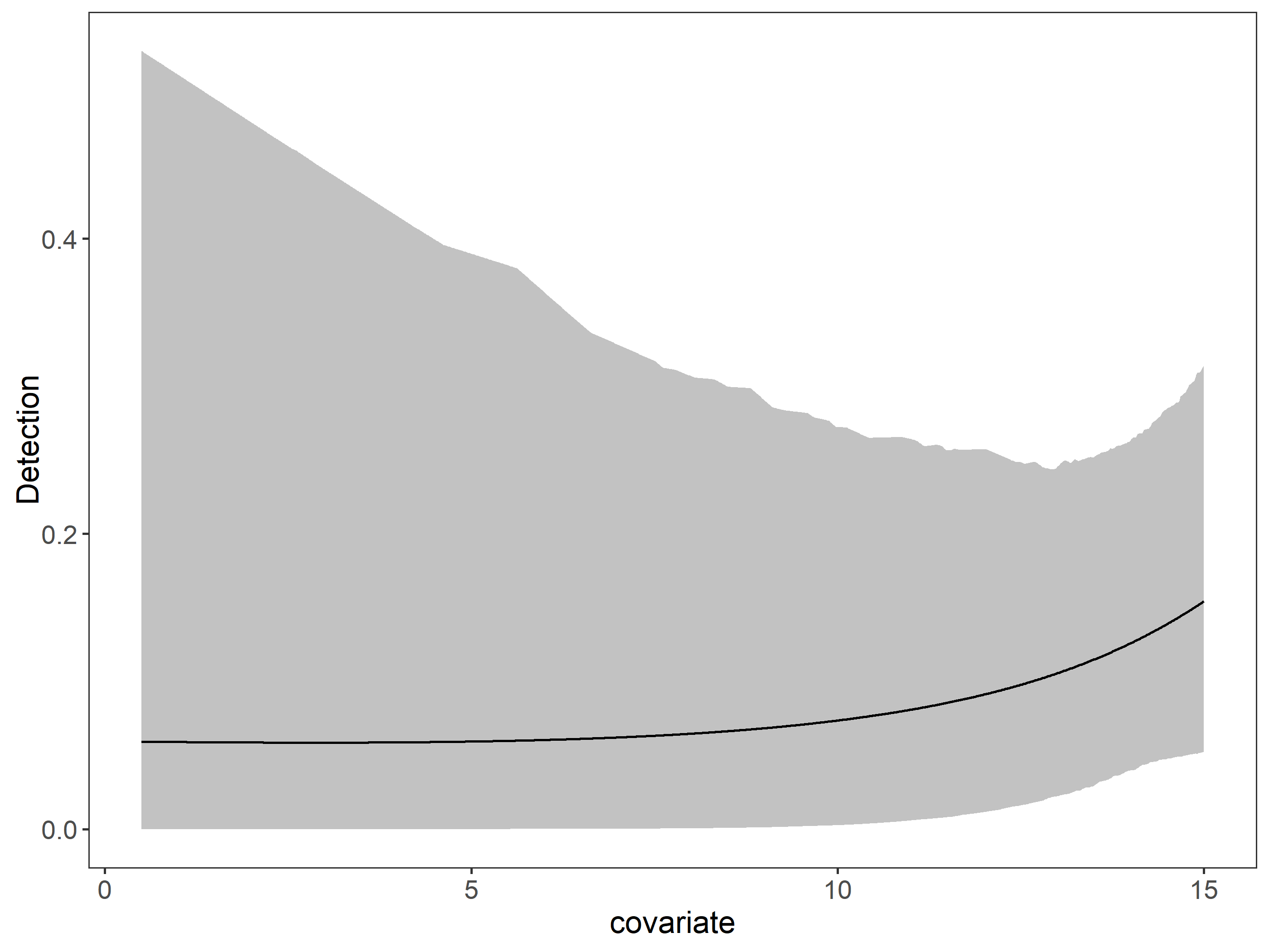
We’ll now we fit a model with fixed effects of percent tree cover road density and cattle density (per_tree_cov, roads and cattle) on occupancy and a effort affecting the detection. In addition, we will include random intercepts by site, since in stacking the data we have pseudoreplication by site. To review, random effects are specified using the approach used in with the lme4 package. For example, a random intercept for each level of the covariate site is specified with the formula component (1|site). Including random effects in a model in ubms usually significantly increases the run time, but at the end is worth the waiting time.

Next we perform model selection.

Code

# fit_0 <- occu(~1~1, data=umf) # unmarked

fit_j0 <- stan_occu(~1~1 + (1|site),
                       data=umf, chains=3, iter=10000, cores=3)
fit_j1 <- stan_occu(~scale(effort) ~1 + (1|site), 
                       data=umf, chains=3, iter=10000)
#> 
#> SAMPLING FOR MODEL 'occu' NOW (CHAIN 1).
#> Chain 1: 
#> Chain 1: Gradient evaluation took 0.00015 seconds
#> Chain 1: 1000 transitions using 10 leapfrog steps per transition would take 1.5 seconds.
#> Chain 1: Adjust your expectations accordingly!
#> Chain 1: 
#> Chain 1: 
#> Chain 1: Iteration:    1 / 10000 [  0%]  (Warmup)
#> Chain 1: Iteration: 1000 / 10000 [ 10%]  (Warmup)
#> Chain 1: Iteration: 2000 / 10000 [ 20%]  (Warmup)
#> Chain 1: Iteration: 3000 / 10000 [ 30%]  (Warmup)
#> Chain 1: Iteration: 4000 / 10000 [ 40%]  (Warmup)
#> Chain 1: Iteration: 5000 / 10000 [ 50%]  (Warmup)
#> Chain 1: Iteration: 5001 / 10000 [ 50%]  (Sampling)
#> Chain 1: Iteration: 6000 / 10000 [ 60%]  (Sampling)
#> Chain 1: Iteration: 7000 / 10000 [ 70%]  (Sampling)
#> Chain 1: Iteration: 8000 / 10000 [ 80%]  (Sampling)
#> Chain 1: Iteration: 9000 / 10000 [ 90%]  (Sampling)
#> Chain 1: Iteration: 10000 / 10000 [100%]  (Sampling)
#> Chain 1: 
#> Chain 1:  Elapsed Time: 10.893 seconds (Warm-up)
#> Chain 1:                15.543 seconds (Sampling)
#> Chain 1:                26.436 seconds (Total)
#> Chain 1: 
#> 
#> SAMPLING FOR MODEL 'occu' NOW (CHAIN 2).
#> Chain 2: 
#> Chain 2: Gradient evaluation took 9.2e-05 seconds
#> Chain 2: 1000 transitions using 10 leapfrog steps per transition would take 0.92 seconds.
#> Chain 2: Adjust your expectations accordingly!
#> Chain 2: 
#> Chain 2: 
#> Chain 2: Iteration:    1 / 10000 [  0%]  (Warmup)
#> Chain 2: Iteration: 1000 / 10000 [ 10%]  (Warmup)
#> Chain 2: Iteration: 2000 / 10000 [ 20%]  (Warmup)
#> Chain 2: Iteration: 3000 / 10000 [ 30%]  (Warmup)
#> Chain 2: Iteration: 4000 / 10000 [ 40%]  (Warmup)
#> Chain 2: Iteration: 5000 / 10000 [ 50%]  (Warmup)
#> Chain 2: Iteration: 5001 / 10000 [ 50%]  (Sampling)
#> Chain 2: Iteration: 6000 / 10000 [ 60%]  (Sampling)
#> Chain 2: Iteration: 7000 / 10000 [ 70%]  (Sampling)
#> Chain 2: Iteration: 8000 / 10000 [ 80%]  (Sampling)
#> Chain 2: Iteration: 9000 / 10000 [ 90%]  (Sampling)
#> Chain 2: Iteration: 10000 / 10000 [100%]  (Sampling)
#> Chain 2: 
#> Chain 2:  Elapsed Time: 13.274 seconds (Warm-up)
#> Chain 2:                16.311 seconds (Sampling)
#> Chain 2:                29.585 seconds (Total)
#> Chain 2: 
#> 
#> SAMPLING FOR MODEL 'occu' NOW (CHAIN 3).
#> Chain 3: 
#> Chain 3: Gradient evaluation took 8.8e-05 seconds
#> Chain 3: 1000 transitions using 10 leapfrog steps per transition would take 0.88 seconds.
#> Chain 3: Adjust your expectations accordingly!
#> Chain 3: 
#> Chain 3: 
#> Chain 3: Iteration:    1 / 10000 [  0%]  (Warmup)
#> Chain 3: Iteration: 1000 / 10000 [ 10%]  (Warmup)
#> Chain 3: Iteration: 2000 / 10000 [ 20%]  (Warmup)
#> Chain 3: Iteration: 3000 / 10000 [ 30%]  (Warmup)
#> Chain 3: Iteration: 4000 / 10000 [ 40%]  (Warmup)
#> Chain 3: Iteration: 5000 / 10000 [ 50%]  (Warmup)
#> Chain 3: Iteration: 5001 / 10000 [ 50%]  (Sampling)
#> Chain 3: Iteration: 6000 / 10000 [ 60%]  (Sampling)
#> Chain 3: Iteration: 7000 / 10000 [ 70%]  (Sampling)
#> Chain 3: Iteration: 8000 / 10000 [ 80%]  (Sampling)
#> Chain 3: Iteration: 9000 / 10000 [ 90%]  (Sampling)
#> Chain 3: Iteration: 10000 / 10000 [100%]  (Sampling)
#> Chain 3: 
#> Chain 3:  Elapsed Time: 12.722 seconds (Warm-up)
#> Chain 3:                11.397 seconds (Sampling)
#> Chain 3:                24.119 seconds (Total)
#> Chain 3:
fit_j2 <- stan_occu(~scale(effort) ~scale(per_tree_cov) + (1|site), 
                       data=umf, chains=3, iter=10000)
#> 
#> SAMPLING FOR MODEL 'occu' NOW (CHAIN 1).
#> Chain 1: 
#> Chain 1: Gradient evaluation took 8.9e-05 seconds
#> Chain 1: 1000 transitions using 10 leapfrog steps per transition would take 0.89 seconds.
#> Chain 1: Adjust your expectations accordingly!
#> Chain 1: 
#> Chain 1: 
#> Chain 1: Iteration:    1 / 10000 [  0%]  (Warmup)
#> Chain 1: Iteration: 1000 / 10000 [ 10%]  (Warmup)
#> Chain 1: Iteration: 2000 / 10000 [ 20%]  (Warmup)
#> Chain 1: Iteration: 3000 / 10000 [ 30%]  (Warmup)
#> Chain 1: Iteration: 4000 / 10000 [ 40%]  (Warmup)
#> Chain 1: Iteration: 5000 / 10000 [ 50%]  (Warmup)
#> Chain 1: Iteration: 5001 / 10000 [ 50%]  (Sampling)
#> Chain 1: Iteration: 6000 / 10000 [ 60%]  (Sampling)
#> Chain 1: Iteration: 7000 / 10000 [ 70%]  (Sampling)
#> Chain 1: Iteration: 8000 / 10000 [ 80%]  (Sampling)
#> Chain 1: Iteration: 9000 / 10000 [ 90%]  (Sampling)
#> Chain 1: Iteration: 10000 / 10000 [100%]  (Sampling)
#> Chain 1: 
#> Chain 1:  Elapsed Time: 18.78 seconds (Warm-up)
#> Chain 1:                155.225 seconds (Sampling)
#> Chain 1:                174.005 seconds (Total)
#> Chain 1: 
#> 
#> SAMPLING FOR MODEL 'occu' NOW (CHAIN 2).
#> Chain 2: 
#> Chain 2: Gradient evaluation took 9e-05 seconds
#> Chain 2: 1000 transitions using 10 leapfrog steps per transition would take 0.9 seconds.
#> Chain 2: Adjust your expectations accordingly!
#> Chain 2: 
#> Chain 2: 
#> Chain 2: Iteration:    1 / 10000 [  0%]  (Warmup)
#> Chain 2: Iteration: 1000 / 10000 [ 10%]  (Warmup)
#> Chain 2: Iteration: 2000 / 10000 [ 20%]  (Warmup)
#> Chain 2: Iteration: 3000 / 10000 [ 30%]  (Warmup)
#> Chain 2: Iteration: 4000 / 10000 [ 40%]  (Warmup)
#> Chain 2: Iteration: 5000 / 10000 [ 50%]  (Warmup)
#> Chain 2: Iteration: 5001 / 10000 [ 50%]  (Sampling)
#> Chain 2: Iteration: 6000 / 10000 [ 60%]  (Sampling)
#> Chain 2: Iteration: 7000 / 10000 [ 70%]  (Sampling)
#> Chain 2: Iteration: 8000 / 10000 [ 80%]  (Sampling)
#> Chain 2: Iteration: 9000 / 10000 [ 90%]  (Sampling)
#> Chain 2: Iteration: 10000 / 10000 [100%]  (Sampling)
#> Chain 2: 
#> Chain 2:  Elapsed Time: 13.014 seconds (Warm-up)
#> Chain 2:                13.599 seconds (Sampling)
#> Chain 2:                26.613 seconds (Total)
#> Chain 2: 
#> 
#> SAMPLING FOR MODEL 'occu' NOW (CHAIN 3).
#> Chain 3: 
#> Chain 3: Gradient evaluation took 8.7e-05 seconds
#> Chain 3: 1000 transitions using 10 leapfrog steps per transition would take 0.87 seconds.
#> Chain 3: Adjust your expectations accordingly!
#> Chain 3: 
#> Chain 3: 
#> Chain 3: Iteration:    1 / 10000 [  0%]  (Warmup)
#> Chain 3: Iteration: 1000 / 10000 [ 10%]  (Warmup)
#> Chain 3: Iteration: 2000 / 10000 [ 20%]  (Warmup)
#> Chain 3: Iteration: 3000 / 10000 [ 30%]  (Warmup)
#> Chain 3: Iteration: 4000 / 10000 [ 40%]  (Warmup)
#> Chain 3: Iteration: 5000 / 10000 [ 50%]  (Warmup)
#> Chain 3: Iteration: 5001 / 10000 [ 50%]  (Sampling)
#> Chain 3: Iteration: 6000 / 10000 [ 60%]  (Sampling)
#> Chain 3: Iteration: 7000 / 10000 [ 70%]  (Sampling)
#> Chain 3: Iteration: 8000 / 10000 [ 80%]  (Sampling)
#> Chain 3: Iteration: 9000 / 10000 [ 90%]  (Sampling)
#> Chain 3: Iteration: 10000 / 10000 [100%]  (Sampling)
#> Chain 3: 
#> Chain 3:  Elapsed Time: 17.036 seconds (Warm-up)
#> Chain 3:                18.42 seconds (Sampling)
#> Chain 3:                35.456 seconds (Total)
#> Chain 3:
fit_j3 <- stan_occu(~scale(effort) ~scale(roads) + (1|site), 
                       data=umf, chains=3, iter=10000)
#> 
#> SAMPLING FOR MODEL 'occu' NOW (CHAIN 1).
#> Chain 1: 
#> Chain 1: Gradient evaluation took 9e-05 seconds
#> Chain 1: 1000 transitions using 10 leapfrog steps per transition would take 0.9 seconds.
#> Chain 1: Adjust your expectations accordingly!
#> Chain 1: 
#> Chain 1: 
#> Chain 1: Iteration:    1 / 10000 [  0%]  (Warmup)
#> Chain 1: Iteration: 1000 / 10000 [ 10%]  (Warmup)
#> Chain 1: Iteration: 2000 / 10000 [ 20%]  (Warmup)
#> Chain 1: Iteration: 3000 / 10000 [ 30%]  (Warmup)
#> Chain 1: Iteration: 4000 / 10000 [ 40%]  (Warmup)
#> Chain 1: Iteration: 5000 / 10000 [ 50%]  (Warmup)
#> Chain 1: Iteration: 5001 / 10000 [ 50%]  (Sampling)
#> Chain 1: Iteration: 6000 / 10000 [ 60%]  (Sampling)
#> Chain 1: Iteration: 7000 / 10000 [ 70%]  (Sampling)
#> Chain 1: Iteration: 8000 / 10000 [ 80%]  (Sampling)
#> Chain 1: Iteration: 9000 / 10000 [ 90%]  (Sampling)
#> Chain 1: Iteration: 10000 / 10000 [100%]  (Sampling)
#> Chain 1: 
#> Chain 1:  Elapsed Time: 9.354 seconds (Warm-up)
#> Chain 1:                12.978 seconds (Sampling)
#> Chain 1:                22.332 seconds (Total)
#> Chain 1: 
#> 
#> SAMPLING FOR MODEL 'occu' NOW (CHAIN 2).
#> Chain 2: 
#> Chain 2: Gradient evaluation took 0.000157 seconds
#> Chain 2: 1000 transitions using 10 leapfrog steps per transition would take 1.57 seconds.
#> Chain 2: Adjust your expectations accordingly!
#> Chain 2: 
#> Chain 2: 
#> Chain 2: Iteration:    1 / 10000 [  0%]  (Warmup)
#> Chain 2: Iteration: 1000 / 10000 [ 10%]  (Warmup)
#> Chain 2: Iteration: 2000 / 10000 [ 20%]  (Warmup)
#> Chain 2: Iteration: 3000 / 10000 [ 30%]  (Warmup)
#> Chain 2: Iteration: 4000 / 10000 [ 40%]  (Warmup)
#> Chain 2: Iteration: 5000 / 10000 [ 50%]  (Warmup)
#> Chain 2: Iteration: 5001 / 10000 [ 50%]  (Sampling)
#> Chain 2: Iteration: 6000 / 10000 [ 60%]  (Sampling)
#> Chain 2: Iteration: 7000 / 10000 [ 70%]  (Sampling)
#> Chain 2: Iteration: 8000 / 10000 [ 80%]  (Sampling)
#> Chain 2: Iteration: 9000 / 10000 [ 90%]  (Sampling)
#> Chain 2: Iteration: 10000 / 10000 [100%]  (Sampling)
#> Chain 2: 
#> Chain 2:  Elapsed Time: 12.283 seconds (Warm-up)
#> Chain 2:                15.241 seconds (Sampling)
#> Chain 2:                27.524 seconds (Total)
#> Chain 2: 
#> 
#> SAMPLING FOR MODEL 'occu' NOW (CHAIN 3).
#> Chain 3: 
#> Chain 3: Gradient evaluation took 0.000103 seconds
#> Chain 3: 1000 transitions using 10 leapfrog steps per transition would take 1.03 seconds.
#> Chain 3: Adjust your expectations accordingly!
#> Chain 3: 
#> Chain 3: 
#> Chain 3: Iteration:    1 / 10000 [  0%]  (Warmup)
#> Chain 3: Iteration: 1000 / 10000 [ 10%]  (Warmup)
#> Chain 3: Iteration: 2000 / 10000 [ 20%]  (Warmup)
#> Chain 3: Iteration: 3000 / 10000 [ 30%]  (Warmup)
#> Chain 3: Iteration: 4000 / 10000 [ 40%]  (Warmup)
#> Chain 3: Iteration: 5000 / 10000 [ 50%]  (Warmup)
#> Chain 3: Iteration: 5001 / 10000 [ 50%]  (Sampling)
#> Chain 3: Iteration: 6000 / 10000 [ 60%]  (Sampling)
#> Chain 3: Iteration: 7000 / 10000 [ 70%]  (Sampling)
#> Chain 3: Iteration: 8000 / 10000 [ 80%]  (Sampling)
#> Chain 3: Iteration: 9000 / 10000 [ 90%]  (Sampling)
#> Chain 3: Iteration: 10000 / 10000 [100%]  (Sampling)
#> Chain 3: 
#> Chain 3:  Elapsed Time: 25.409 seconds (Warm-up)
#> Chain 3:                18.233 seconds (Sampling)
#> Chain 3:                43.642 seconds (Total)
#> Chain 3:
fit_j4 <- stan_occu(~scale(effort) ~scale(cattle) + (1|site), 
                       data=umf, chains=3, iter=10000)
#> 
#> SAMPLING FOR MODEL 'occu' NOW (CHAIN 1).
#> Chain 1: 
#> Chain 1: Gradient evaluation took 9.1e-05 seconds
#> Chain 1: 1000 transitions using 10 leapfrog steps per transition would take 0.91 seconds.
#> Chain 1: Adjust your expectations accordingly!
#> Chain 1: 
#> Chain 1: 
#> Chain 1: Iteration:    1 / 10000 [  0%]  (Warmup)
#> Chain 1: Iteration: 1000 / 10000 [ 10%]  (Warmup)
#> Chain 1: Iteration: 2000 / 10000 [ 20%]  (Warmup)
#> Chain 1: Iteration: 3000 / 10000 [ 30%]  (Warmup)
#> Chain 1: Iteration: 4000 / 10000 [ 40%]  (Warmup)
#> Chain 1: Iteration: 5000 / 10000 [ 50%]  (Warmup)
#> Chain 1: Iteration: 5001 / 10000 [ 50%]  (Sampling)
#> Chain 1: Iteration: 6000 / 10000 [ 60%]  (Sampling)
#> Chain 1: Iteration: 7000 / 10000 [ 70%]  (Sampling)
#> Chain 1: Iteration: 8000 / 10000 [ 80%]  (Sampling)
#> Chain 1: Iteration: 9000 / 10000 [ 90%]  (Sampling)
#> Chain 1: Iteration: 10000 / 10000 [100%]  (Sampling)
#> Chain 1: 
#> Chain 1:  Elapsed Time: 12.766 seconds (Warm-up)
#> Chain 1:                21.386 seconds (Sampling)
#> Chain 1:                34.152 seconds (Total)
#> Chain 1: 
#> 
#> SAMPLING FOR MODEL 'occu' NOW (CHAIN 2).
#> Chain 2: 
#> Chain 2: Gradient evaluation took 9.8e-05 seconds
#> Chain 2: 1000 transitions using 10 leapfrog steps per transition would take 0.98 seconds.
#> Chain 2: Adjust your expectations accordingly!
#> Chain 2: 
#> Chain 2: 
#> Chain 2: Iteration:    1 / 10000 [  0%]  (Warmup)
#> Chain 2: Iteration: 1000 / 10000 [ 10%]  (Warmup)
#> Chain 2: Iteration: 2000 / 10000 [ 20%]  (Warmup)
#> Chain 2: Iteration: 3000 / 10000 [ 30%]  (Warmup)
#> Chain 2: Iteration: 4000 / 10000 [ 40%]  (Warmup)
#> Chain 2: Iteration: 5000 / 10000 [ 50%]  (Warmup)
#> Chain 2: Iteration: 5001 / 10000 [ 50%]  (Sampling)
#> Chain 2: Iteration: 6000 / 10000 [ 60%]  (Sampling)
#> Chain 2: Iteration: 7000 / 10000 [ 70%]  (Sampling)
#> Chain 2: Iteration: 8000 / 10000 [ 80%]  (Sampling)
#> Chain 2: Iteration: 9000 / 10000 [ 90%]  (Sampling)
#> Chain 2: Iteration: 10000 / 10000 [100%]  (Sampling)
#> Chain 2: 
#> Chain 2:  Elapsed Time: 13.028 seconds (Warm-up)
#> Chain 2:                11.989 seconds (Sampling)
#> Chain 2:                25.017 seconds (Total)
#> Chain 2: 
#> 
#> SAMPLING FOR MODEL 'occu' NOW (CHAIN 3).
#> Chain 3: 
#> Chain 3: Gradient evaluation took 8.8e-05 seconds
#> Chain 3: 1000 transitions using 10 leapfrog steps per transition would take 0.88 seconds.
#> Chain 3: Adjust your expectations accordingly!
#> Chain 3: 
#> Chain 3: 
#> Chain 3: Iteration:    1 / 10000 [  0%]  (Warmup)
#> Chain 3: Iteration: 1000 / 10000 [ 10%]  (Warmup)
#> Chain 3: Iteration: 2000 / 10000 [ 20%]  (Warmup)
#> Chain 3: Iteration: 3000 / 10000 [ 30%]  (Warmup)
#> Chain 3: Iteration: 4000 / 10000 [ 40%]  (Warmup)
#> Chain 3: Iteration: 5000 / 10000 [ 50%]  (Warmup)
#> Chain 3: Iteration: 5001 / 10000 [ 50%]  (Sampling)
#> Chain 3: Iteration: 6000 / 10000 [ 60%]  (Sampling)
#> Chain 3: Iteration: 7000 / 10000 [ 70%]  (Sampling)
#> Chain 3: Iteration: 8000 / 10000 [ 80%]  (Sampling)
#> Chain 3: Iteration: 9000 / 10000 [ 90%]  (Sampling)
#> Chain 3: Iteration: 10000 / 10000 [100%]  (Sampling)
#> Chain 3: 
#> Chain 3:  Elapsed Time: 17.715 seconds (Warm-up)
#> Chain 3:                19.229 seconds (Sampling)
#> Chain 3:                36.944 seconds (Total)
#> Chain 3:
# compare
models <- list(Null = fit_j0,
                effort = fit_j1,
                effort_treecov = fit_j2,
                effort_road = fit_j3,
                effort_cattle = fit_j4)

mods <- fitList(fits = models)


## see model selection as a table
datatable( 
  round(modSel(mods), 3)
  )

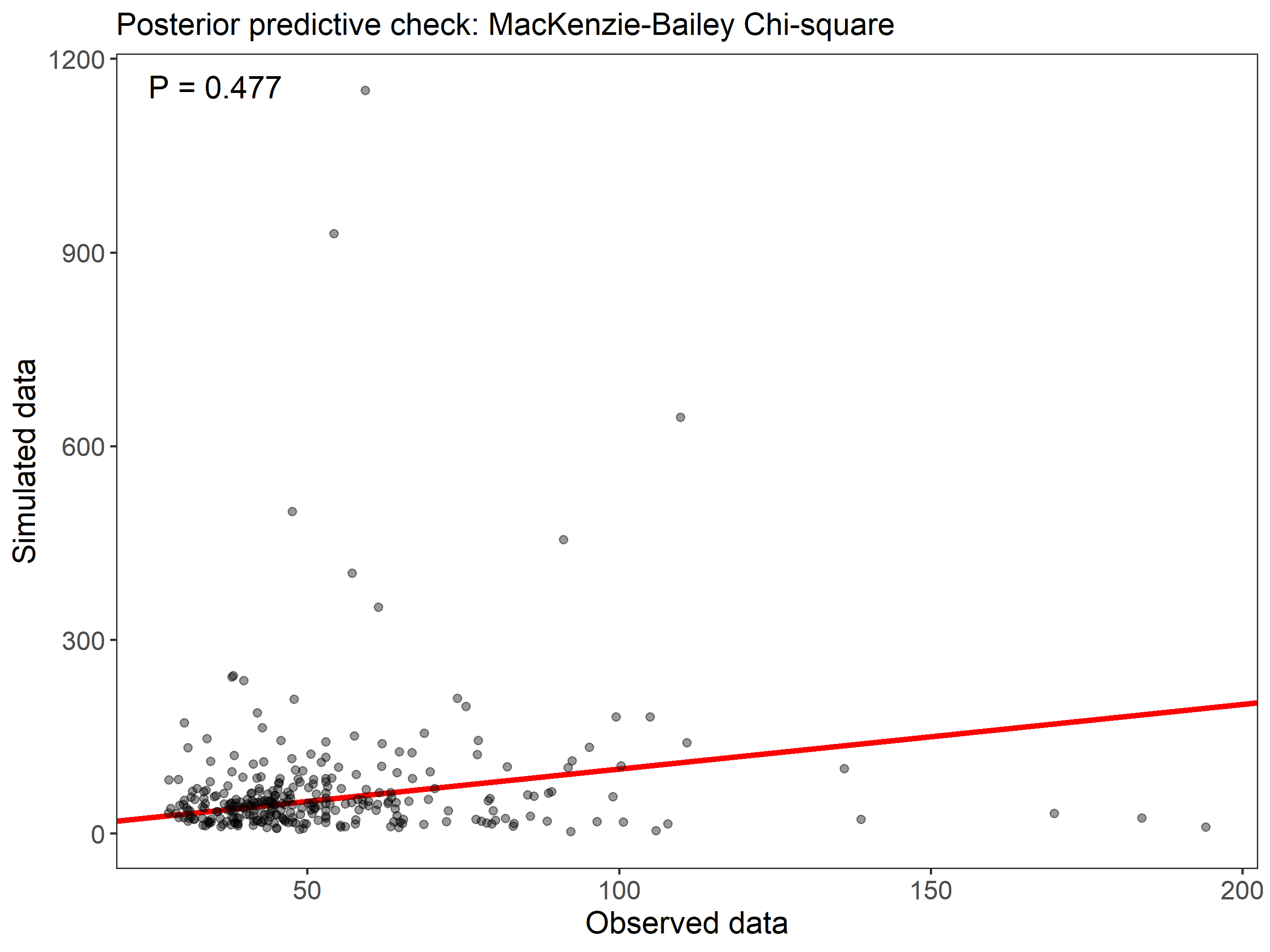
Instead of AIC, models are compared using leave-one-out cross-validation (LOO) (Vehtari, Gelman, and Gabry 2017) via the loo package. Based on this cross-validation, the expected predictive accuracy (elpd) for each model is calculated. The model with the largest elpd (effort_cattle) performed best. The looic value is analogous to AIC.

Code

loo(fit_j4)
#> 
#> Computed from 15000 by 53 log-likelihood matrix.
#> 
#>          Estimate   SE
#> elpd_loo    -54.7 13.5
#> p_loo         4.4  1.0
#> looic       109.3 27.0
#> ------
#> MCSE of elpd_loo is 0.1.
#> MCSE and ESS estimates assume MCMC draws (r_eff in [0.0, 0.8]).
#> 
#> All Pareto k estimates are good (k < 0.7).
#> See help('pareto-k-diagnostic') for details.

Best model is effort_cattle (fit_j4) which has effort on detection and percent tree cover on occupancy.

Code

fit_j4
#> 
#> Call:
#> stan_occu(formula = ~scale(effort) ~ scale(cattle) + (1 | site), 
#>     data = umf, chains = 3, iter = 10000)
#> 
#> Occupancy (logit-scale):
#>                Estimate    SD    2.5% 97.5% n_eff Rhat
#> (Intercept)       -1.33 0.783 -2.6781 0.399   508 1.01
#> scale(cattle)     -1.30 1.091 -3.7546 0.351   466 1.01
#> sigma [1|site]     0.74 0.745  0.0451 2.661   219 1.02
#> 
#> Detection (logit-scale):
#>               Estimate    SD  2.5%  97.5% n_eff Rhat
#> (Intercept)     -1.625 0.475 -2.67 -0.771  2219 1.00
#> scale(effort)    0.343 0.353 -0.31  1.056   678 1.01
#> 
#> LOOIC: 109.302
#> Runtime: 96.113 sec

Looking at the summary of fit_j4, we conclude MCMC chains have converged if all R^>1.05 To visualize convergence, look at the traceplots:

Code

traceplot(fit_j4, pars=c("beta_state", "beta_det"))

Evaluate model fit

Statistic should be near 0.5 if the model fits well.

Code

# eval
fit_top_gof <- gof(fit_j4, draws=300, quiet=TRUE)
fit_top_gof
#> MacKenzie-Bailey Chi-square 
#> Point estimate = 53.154
#> Posterior predictive p = 0.477

plot(fit_top_gof)

Model inference

Effort in detection and cattle density in occupancy

Code

ubms::plot_effects(fit_j4, "det")

Code

ubms::plot_effects(fit_j4, "state")

Comparing occupancy between years

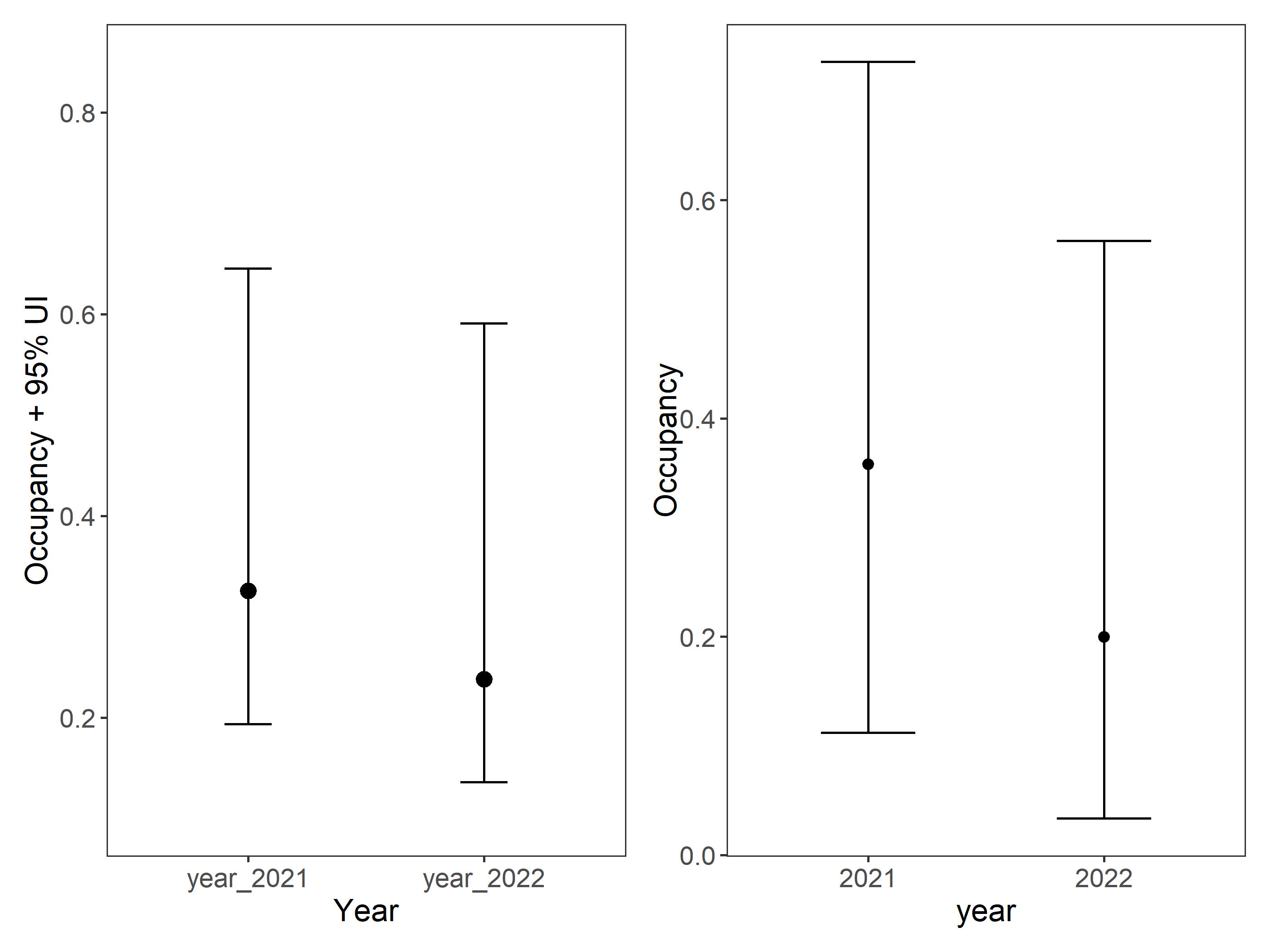
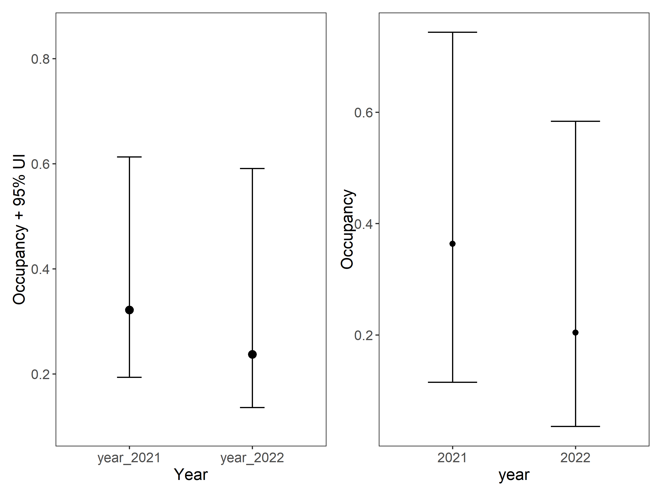
Using the posterior_predict function in ubms, you can generate an equivalent posterior distribution of z, and latter to do a post-hoc analyses to test for a difference in mean occupancy probability between sites 2021 and sites 2022.

Code

zpost <- posterior_predict(fit_j4, "z", draws=1000)
dim(zpost)
#> [1] 1000   55

year_2021 <- rowMeans(zpost[,1:32], na.rm=TRUE)
year_2022 <- rowMeans(zpost[,33:55], na.rm=TRUE)

plot_dat <- rbind(data.frame(group="year_2021", occ=mean(year_2021),
                             lower=quantile(year_2021, 0.025),
                             upper=quantile(year_2021, 0.975)),
                  data.frame(group="year_2022", occ=mean(year_2022),
                             lower=quantile(year_2022, 0.025),
                             upper=quantile(year_2022, 0.975)))

# Now plot the posterior distributions of the two means:


ggplot(plot_dat, aes(x=group, y=occ)) +
  geom_errorbar(aes(ymin=lower, ymax=upper), width=0.2) +
  geom_point(size=3) +
  ylim(0,1) +
  labs(x="Year", y="Occupancy + 95% UI") +
  theme_bw() +
  theme(panel.grid.major=element_blank(), panel.grid.minor=element_blank(),
        axis.text=element_text(size=12), axis.title=element_text(size=14))

It seems the difference in mean occupancy probability between years is not significant.

Package Citation

Code

pkgs <- cite_packages(output = "paragraph", out.dir = ".") #knitr::kable(pkgs)
pkgs

We used R version 4.3.2 (R Core Team 2023) and the following R packages: camtrapR v. 2.3.0 (Niedballa et al. 2016), devtools v. 2.4.5 (Wickham et al. 2022), DT v. 0.33 (Xie, Cheng, and Tan 2024), elevatr v. 0.99.0 (Hollister et al. 2023), kableExtra v. 1.4.0 (Zhu 2024), lme4 v. 1.1.35.5 (Bates et al. 2015), mapview v. 2.11.2 (Appelhans et al. 2023), patchwork v. 1.3.0 (Pedersen 2024), quarto v. 1.4.4 (Allaire and Dervieux 2024), rmarkdown v. 2.28 (Xie, Allaire, and Grolemund 2018; Xie, Dervieux, and Riederer 2020; Allaire et al. 2024), sf v. 1.0.17 (Pebesma 2018; Pebesma and Bivand 2023), styler v. 1.10.3 (Müller and Walthert 2024), terra v. 1.7.78 (Hijmans 2024), tidyverse v. 2.0.0 (Wickham et al. 2019), ubms v. 1.2.7 (Kellner et al. 2021).

Sesion info

Session info

#> ─ Session info ───────────────────────────────────────────────────────────────────────────────────────────────────────
#>  setting  value
#>  version  R version 4.3.2 (2023-10-31 ucrt)
#>  os       Windows 10 x64 (build 19042)
#>  system   x86_64, mingw32
#>  ui       RTerm
#>  language (EN)
#>  collate  Spanish_Colombia.utf8
#>  ctype    Spanish_Colombia.utf8
#>  tz       America/Bogota
#>  date     2024-10-31
#>  pandoc   3.2 @ C:/Program Files/RStudio/resources/app/bin/quarto/bin/tools/ (via rmarkdown)
#> 
#> ─ Packages ───────────────────────────────────────────────────────────────────────────────────────────────────────────
#>  ! package           * version  date (UTC) lib source
#>    abind               1.4-8    2024-09-12 [1] CRAN (R 4.3.2)
#>    archive             1.1.9    2024-09-12 [1] CRAN (R 4.3.2)
#>    backports           1.5.0    2024-05-23 [1] CRAN (R 4.3.3)
#>    base64enc           0.1-3    2015-07-28 [1] CRAN (R 4.3.1)
#>    bit                 4.5.0    2024-09-20 [1] CRAN (R 4.3.3)
#>    bit64               4.5.2    2024-09-22 [1] CRAN (R 4.3.3)
#>    boot                1.3-31   2024-08-28 [2] CRAN (R 4.3.3)
#>    brew                1.0-10   2023-12-16 [1] CRAN (R 4.3.2)
#>    bslib               0.8.0    2024-07-29 [1] CRAN (R 4.3.3)
#>    cachem              1.1.0    2024-05-16 [1] CRAN (R 4.3.3)
#>    camtrapR          * 2.3.0    2024-02-26 [1] CRAN (R 4.3.3)
#>    cellranger          1.1.0    2016-07-27 [1] CRAN (R 4.3.2)
#>    checkmate           2.3.2    2024-07-29 [1] CRAN (R 4.3.3)
#>    class               7.3-22   2023-05-03 [2] CRAN (R 4.3.2)
#>    classInt            0.4-10   2023-09-05 [1] CRAN (R 4.3.2)
#>    cli                 3.6.3    2024-06-21 [1] CRAN (R 4.3.3)
#>    codetools           0.2-20   2024-03-31 [2] CRAN (R 4.3.3)
#>    colorspace          2.1-1    2024-07-26 [1] CRAN (R 4.3.3)
#>    crayon              1.5.3    2024-06-20 [1] CRAN (R 4.3.3)
#>    crosstalk           1.2.1    2023-11-23 [1] CRAN (R 4.3.2)
#>    curl                5.2.3    2024-09-20 [1] CRAN (R 4.3.3)
#>    data.table          1.16.0   2024-08-27 [1] CRAN (R 4.3.3)
#>    DBI                 1.2.3    2024-06-02 [1] CRAN (R 4.3.3)
#>    devtools            2.4.5    2022-10-11 [1] CRAN (R 4.3.2)
#>    digest              0.6.37   2024-08-19 [1] CRAN (R 4.3.3)
#>    distributional      0.4.0    2024-02-07 [1] CRAN (R 4.3.2)
#>    dplyr             * 1.1.4    2023-11-17 [1] CRAN (R 4.3.2)
#>    DT                * 0.33     2024-04-04 [1] CRAN (R 4.3.3)
#>    e1071               1.7-14   2023-12-06 [1] CRAN (R 4.3.2)
#>    elevatr           * 0.99.0   2023-09-12 [1] CRAN (R 4.3.2)
#>    ellipsis            0.3.2    2021-04-29 [1] CRAN (R 4.3.2)
#>    evaluate            0.24.0   2024-06-10 [1] CRAN (R 4.3.3)
#>    fansi               1.0.6    2023-12-08 [1] CRAN (R 4.3.2)
#>    farver              2.1.2    2024-05-13 [1] CRAN (R 4.3.3)
#>    fastmap             1.2.0    2024-05-15 [1] CRAN (R 4.3.3)
#>    forcats           * 1.0.0    2023-01-29 [1] CRAN (R 4.3.2)
#>    fs                  1.6.4    2024-04-25 [1] CRAN (R 4.3.3)
#>    generics            0.1.3    2022-07-05 [1] CRAN (R 4.3.2)
#>    ggplot2           * 3.5.1    2024-04-23 [1] CRAN (R 4.3.3)
#>    glue                1.8.0    2024-09-30 [1] CRAN (R 4.3.3)
#>    grateful          * 0.2.10   2024-09-04 [1] CRAN (R 4.3.3)
#>    gridExtra           2.3      2017-09-09 [1] CRAN (R 4.3.2)
#>    gtable              0.3.5    2024-04-22 [1] CRAN (R 4.3.3)
#>    hms                 1.1.3    2023-03-21 [1] CRAN (R 4.3.2)
#>    htmltools           0.5.8.1  2024-04-04 [1] CRAN (R 4.3.3)
#>    htmlwidgets         1.6.4    2023-12-06 [1] CRAN (R 4.3.2)
#>    httpuv              1.6.15   2024-03-26 [1] CRAN (R 4.3.3)
#>    inline              0.3.19   2021-05-31 [1] CRAN (R 4.3.2)
#>    jquerylib           0.1.4    2021-04-26 [1] CRAN (R 4.3.2)
#>    jsonlite            1.8.9    2024-09-20 [1] CRAN (R 4.3.3)
#>    kableExtra        * 1.4.0    2024-01-24 [1] CRAN (R 4.3.3)
#>    KernSmooth          2.23-24  2024-05-17 [2] CRAN (R 4.3.3)
#>    knitr               1.48     2024-07-07 [1] CRAN (R 4.3.3)
#>    labeling            0.4.3    2023-08-29 [1] CRAN (R 4.3.1)
#>    later               1.3.2    2023-12-06 [1] CRAN (R 4.3.2)
#>    lattice             0.22-6   2024-03-20 [1] CRAN (R 4.3.3)
#>    leafem              0.2.3    2023-09-17 [1] CRAN (R 4.3.2)
#>    leaflet             2.2.2    2024-03-26 [1] CRAN (R 4.3.3)
#>    leaflet.providers   2.0.0    2023-10-17 [1] CRAN (R 4.3.2)
#>    leafpop             0.1.0    2021-05-22 [1] CRAN (R 4.3.2)
#>    lifecycle           1.0.4    2023-11-07 [1] CRAN (R 4.3.2)
#>    lme4              * 1.1-35.5 2024-07-03 [1] CRAN (R 4.3.3)
#>    loo                 2.8.0    2024-07-03 [1] CRAN (R 4.3.3)
#>    lubridate         * 1.9.3    2023-09-27 [1] CRAN (R 4.3.2)
#>    magrittr            2.0.3    2022-03-30 [1] CRAN (R 4.3.2)
#>    mapview           * 2.11.2   2023-10-13 [1] CRAN (R 4.3.2)
#>    MASS                7.3-60   2023-05-04 [2] CRAN (R 4.3.2)
#>    Matrix            * 1.6-1.1  2023-09-18 [2] CRAN (R 4.3.2)
#>    matrixStats         1.4.1    2024-09-08 [1] CRAN (R 4.3.3)
#>    memoise             2.0.1    2021-11-26 [1] CRAN (R 4.3.2)
#>    mgcv                1.9-1    2023-12-21 [1] CRAN (R 4.3.3)
#>    mime                0.12     2021-09-28 [1] CRAN (R 4.3.1)
#>    miniUI              0.1.1.1  2018-05-18 [1] CRAN (R 4.3.2)
#>    minqa               1.2.8    2024-08-17 [1] CRAN (R 4.3.3)
#>    munsell             0.5.1    2024-04-01 [1] CRAN (R 4.3.3)
#>    mvtnorm             1.3-1    2024-09-03 [1] CRAN (R 4.3.3)
#>    nlme                3.1-166  2024-08-14 [2] CRAN (R 4.3.3)
#>    nloptr              2.1.1    2024-06-25 [1] CRAN (R 4.3.3)
#>    patchwork         * 1.3.0    2024-09-16 [1] CRAN (R 4.3.3)
#>    pbapply             1.7-2    2023-06-27 [1] CRAN (R 4.3.2)
#>    pillar              1.9.0    2023-03-22 [1] CRAN (R 4.3.2)
#>    pkgbuild            1.4.4    2024-03-17 [1] CRAN (R 4.3.3)
#>    pkgconfig           2.0.3    2019-09-22 [1] CRAN (R 4.3.2)
#>    pkgload             1.4.0    2024-06-28 [1] CRAN (R 4.3.3)
#>    png                 0.1-8    2022-11-29 [1] CRAN (R 4.3.1)
#>    posterior           1.6.0    2024-07-03 [1] CRAN (R 4.3.3)
#>    processx            3.8.4    2024-03-16 [1] CRAN (R 4.3.3)
#>    profvis             0.3.8    2023-05-02 [1] CRAN (R 4.3.2)
#>    progressr           0.14.0   2023-08-10 [1] CRAN (R 4.3.2)
#>    promises            1.3.0    2024-04-05 [1] CRAN (R 4.3.3)
#>    proxy               0.4-27   2022-06-09 [1] CRAN (R 4.3.2)
#>    ps                  1.8.0    2024-09-12 [1] CRAN (R 4.3.2)
#>    purrr             * 1.0.2    2023-08-10 [1] CRAN (R 4.3.2)
#>    quarto            * 1.4.4    2024-07-20 [1] CRAN (R 4.3.3)
#>    QuickJSR            1.3.1    2024-07-14 [1] CRAN (R 4.3.3)
#>    R.cache             0.16.0   2022-07-21 [1] CRAN (R 4.3.3)
#>    R.methodsS3         1.8.2    2022-06-13 [1] CRAN (R 4.3.3)
#>    R.oo                1.26.0   2024-01-24 [1] CRAN (R 4.3.3)
#>    R.utils             2.12.3   2023-11-18 [1] CRAN (R 4.3.3)
#>    R6                  2.5.1    2021-08-19 [1] CRAN (R 4.3.2)
#>    raster              3.6-30   2024-10-02 [1] CRAN (R 4.3.3)
#>    rbibutils           2.2.16   2023-10-25 [1] CRAN (R 4.3.3)
#>    Rcpp                1.0.13   2024-07-17 [1] CRAN (R 4.3.3)
#>    RcppNumerical       0.6-0    2023-09-06 [1] CRAN (R 4.3.3)
#>  D RcppParallel        5.1.9    2024-08-19 [1] CRAN (R 4.3.3)
#>    Rdpack              2.6.1    2024-08-06 [1] CRAN (R 4.3.3)
#>    readr             * 2.1.5    2024-01-10 [1] CRAN (R 4.3.2)
#>    readxl            * 1.4.3    2023-07-06 [1] CRAN (R 4.3.2)
#>    reformulas          0.3.0    2024-06-05 [1] CRAN (R 4.3.3)
#>    remotes             2.5.0    2024-03-17 [1] CRAN (R 4.3.3)
#>    renv                1.0.7    2024-04-11 [1] CRAN (R 4.3.3)
#>    rlang               1.1.4    2024-06-04 [1] CRAN (R 4.3.3)
#>    rmarkdown           2.28     2024-08-17 [1] CRAN (R 4.3.3)
#>    RSpectra            0.16-2   2024-07-18 [1] CRAN (R 4.3.3)
#>    rstan               2.32.6   2024-03-05 [1] CRAN (R 4.3.3)
#>    rstantools          2.4.0    2024-01-31 [1] CRAN (R 4.3.2)
#>    rstudioapi          0.16.0   2024-03-24 [1] CRAN (R 4.3.3)
#>    sass                0.4.9    2024-03-15 [1] CRAN (R 4.3.3)
#>    satellite           1.0.5    2024-02-10 [1] CRAN (R 4.3.2)
#>    scales              1.3.0    2023-11-28 [1] CRAN (R 4.3.3)
#>    secr                5.0.0    2024-10-02 [1] CRAN (R 4.3.3)
#>    sessioninfo         1.2.2    2021-12-06 [1] CRAN (R 4.3.2)
#>    sf                * 1.0-17   2024-09-06 [1] CRAN (R 4.3.3)
#>    shiny               1.9.1    2024-08-01 [1] CRAN (R 4.3.3)
#>    sp                  2.1-4    2024-04-30 [1] CRAN (R 4.3.3)
#>    StanHeaders         2.32.10  2024-07-15 [1] CRAN (R 4.3.3)
#>    stringi             1.8.4    2024-05-06 [1] CRAN (R 4.3.3)
#>    stringr           * 1.5.1    2023-11-14 [1] CRAN (R 4.3.2)
#>    styler            * 1.10.3   2024-04-07 [1] CRAN (R 4.3.3)
#>    svglite             2.1.3    2023-12-08 [1] CRAN (R 4.3.2)
#>    systemfonts         1.1.0    2024-05-15 [1] CRAN (R 4.3.3)
#>    tensorA             0.36.2.1 2023-12-13 [1] CRAN (R 4.3.2)
#>    terra             * 1.7-78   2024-05-22 [1] CRAN (R 4.3.3)
#>    tibble            * 3.2.1    2023-03-20 [1] CRAN (R 4.3.2)
#>    tidyr             * 1.3.1    2024-01-24 [1] CRAN (R 4.3.2)
#>    tidyselect          1.2.1    2024-03-11 [1] CRAN (R 4.3.3)
#>    tidyverse         * 2.0.0    2023-02-22 [1] CRAN (R 4.3.2)
#>    timechange          0.3.0    2024-01-18 [1] CRAN (R 4.3.2)
#>    tzdb                0.4.0    2023-05-12 [1] CRAN (R 4.3.2)
#>    ubms              * 1.2.7    2024-10-01 [1] CRAN (R 4.3.3)
#>    units               0.8-5    2023-11-28 [1] CRAN (R 4.3.2)
#>    unmarked          * 1.4.3    2024-09-01 [1] CRAN (R 4.3.3)
#>    urlchecker          1.0.1    2021-11-30 [1] CRAN (R 4.3.2)
#>    usethis             3.0.0    2024-07-29 [1] CRAN (R 4.3.3)
#>    utf8                1.2.4    2023-10-22 [1] CRAN (R 4.3.2)
#>    uuid                1.2-1    2024-07-29 [1] CRAN (R 4.3.3)
#>    V8                  5.0.0    2024-08-16 [1] CRAN (R 4.3.3)
#>    vctrs               0.6.5    2023-12-01 [1] CRAN (R 4.3.2)
#>    viridisLite         0.4.2    2023-05-02 [1] CRAN (R 4.3.2)
#>    vroom               1.6.5    2023-12-05 [1] CRAN (R 4.3.2)
#>    withr               3.0.1    2024-07-31 [1] CRAN (R 4.3.3)
#>    xfun                0.47     2024-08-17 [1] CRAN (R 4.3.3)
#>    xml2                1.3.6    2023-12-04 [1] CRAN (R 4.3.2)
#>    xtable              1.8-4    2019-04-21 [1] CRAN (R 4.3.2)
#>    yaml                2.3.10   2024-07-26 [1] CRAN (R 4.3.3)
#> 
#>  [1] C:/Users/usuario/AppData/Local/R/win-library/4.3
#>  [2] C:/Program Files/R/R-4.3.2/library
#> 
#>  D ── DLL MD5 mismatch, broken installation.
#> 
#> ──────────────────────────────────────────────────────────────────────────────────────────────────────────────────────

References

Allaire, JJ, and Christophe Dervieux. 2024. quarto: R Interface to “Quarto” Markdown Publishing System. https://CRAN.R-project.org/package=quarto.

Allaire, JJ, Yihui Xie, Christophe Dervieux, Jonathan McPherson, Javier Luraschi, Kevin Ushey, Aron Atkins, et al. 2024. rmarkdown: Dynamic Documents for r. https://github.com/rstudio/rmarkdown.

Appelhans, Tim, Florian Detsch, Christoph Reudenbach, and Stefan Woellauer. 2023. mapview: Interactive Viewing of Spatial Data in r. https://CRAN.R-project.org/package=mapview.

Bates, Douglas, Martin Mächler, Ben Bolker, and Steve Walker. 2015. “Fitting Linear Mixed-Effects Models Using lme4.” Journal of Statistical Software 67 (1): 1–48. https://doi.org/10.18637/jss.v067.i01.

Gilbert, Marius, Gaëlle Nicolas, Giusepina Cinardi, Thomas P Van Boeckel, Sophie O Vanwambeke, G R William Wint, and Timothy P Robinson. 2018. “Global distribution data for cattle, buffaloes, horses, sheep, goats, pigs, chickens and ducks in 2010.” Scientific Data 5 (1): 180227. https://doi.org/10.1038/sdata.2018.227.

Hijmans, Robert J. 2024. terra: Spatial Data Analysis. https://CRAN.R-project.org/package=terra.

Hollister, Jeffrey, Tarak Shah, Jakub Nowosad, Alec L. Robitaille, Marcus W. Beck, and Mike Johnson. 2023. elevatr: Access Elevation Data from Various APIs. https://doi.org/10.5281/zenodo.8335450.

Kellner, Kenneth F., Nicholas L. Fowler, Tyler R. Petroelje, Todd M. Kautz, Dean E. Beyer, and Jerrold L. Belant. 2021. “ubms: An R Package for Fitting Hierarchical Occupancy and n-Mixture Abundance Models in a Bayesian Framework.” Methods in Ecology and Evolution 13: 577–84. https://doi.org/10.1111/2041-210X.13777.

Meijer, Johan R, Mark A J Huijbregts, Kees C G J Schotten, and Aafke M Schipper. 2018. “Global patterns of current and future road infrastructure.” Environmental Research Letters 13 (6): 64006. https://doi.org/10.1088/1748-9326/aabd42.

Müller, Kirill, and Lorenz Walthert. 2024. styler: Non-Invasive Pretty Printing of r Code. https://CRAN.R-project.org/package=styler.

Niedballa, Jürgen, Rahel Sollmann, Alexandre Courtiol, and Andreas Wilting. 2016. “camtrapR: An r Package for Efficient Camera Trap Data Management.” Methods in Ecology and Evolution 7 (12): 1457–62. https://doi.org/10.1111/2041-210X.12600.

Pebesma, Edzer. 2018. “Simple Features for R: Standardized Support for Spatial Vector Data.” The R Journal 10 (1): 439–46. https://doi.org/10.32614/RJ-2018-009.

Pebesma, Edzer, and Roger Bivand. 2023. Spatial Data Science: With applications in R. Chapman and Hall/CRC. https://doi.org/10.1201/9780429459016.

Pedersen, Thomas Lin. 2024. patchwork: The Composer of Plots. https://CRAN.R-project.org/package=patchwork.

R Core Team. 2023. R: A Language and Environment for Statistical Computing. Vienna, Austria: R Foundation for Statistical Computing. https://www.R-project.org/.

Wickham, Hadley, Mara Averick, Jennifer Bryan, Winston Chang, Lucy D’Agostino McGowan, Romain François, Garrett Grolemund, et al. 2019. “Welcome to the tidyverse.” Journal of Open Source Software 4 (43): 1686. https://doi.org/10.21105/joss.01686.

Wickham, Hadley, Jim Hester, Winston Chang, and Jennifer Bryan. 2022. devtools: Tools to Make Developing r Packages Easier. https://CRAN.R-project.org/package=devtools.

Xie, Yihui, J. J. Allaire, and Garrett Grolemund. 2018. R Markdown: The Definitive Guide. Boca Raton, Florida: Chapman; Hall/CRC. https://bookdown.org/yihui/rmarkdown.

Xie, Yihui, Joe Cheng, and Xianying Tan. 2024. DT: A Wrapper of the JavaScript Library “DataTables”. https://CRAN.R-project.org/package=DT.

Xie, Yihui, Christophe Dervieux, and Emily Riederer. 2020. R Markdown Cookbook. Boca Raton, Florida: Chapman; Hall/CRC. https://bookdown.org/yihui/rmarkdown-cookbook.

Zhu, Hao. 2024. kableExtra: Construct Complex Table with “kable” and Pipe Syntax. https://CRAN.R-project.org/package=kableExtra.

Citation

BibTeX citation:

@online{j._lizcano2024,
  author = {J. Lizcano, Diego and F. González-Maya, José},
  title = {“{Stacked}” {Models}},
  date = {2024-07-17},
  url = {https://dlizcano.github.io/cametrap/posts/2024-07-17-stackmodel/},
  langid = {en}
}

For attribution, please cite this work as:

J. Lizcano, Diego, and José F. González-Maya. 2024. “‘Stacked’ Models.” July 17, 2024. https://dlizcano.github.io/cametrap/posts/2024-07-17-stackmodel/.

Using random effects with ubms

The “stacked” model

Load packages

Load data

Convert to sf and view the map

Extract site covariates

Select by years and convert to stacked format

First year 2021

Next, the year 2022

Save and fix in excel

Jaguar

Fitting a stacked model for jaguar

Load the data

Look at the data

Create an unmarked frame

Fit models

Fit the Stacked Model

Evaluate model fit

Model inference

Comparing occupancy between years

Package Citation

Sesion info

References

Citation

Using random effects with `ubms`