# 2. Model fitting --------------------------------------------------------
# Fit a non-spatial, single-species occupancy model.
out <- PGOcc(
occ.formula = ~ scale(per_tree_cov) + scale(roads) +
scale(cattle),
det.formula = ~ scale(effort),
data = jaguar.data,
n.samples = 50000,
n.thin = 2,
n.burn = 5000,
n.chains = 3,
n.report = 500
)
#> ----------------------------------------
#> Preparing to run the model
#> ----------------------------------------
#> ----------------------------------------
#> Model description
#> ----------------------------------------
#> Occupancy model with Polya-Gamma latent
#> variable fit with 31 sites.
#>
#> Samples per Chain: 50000
#> Burn-in: 5000
#> Thinning Rate: 2
#> Number of Chains: 3
#> Total Posterior Samples: 67500
#>
#> Source compiled with OpenMP support and model fit using 1 thread(s).
#>
#> ----------------------------------------
#> Chain 1
#> ----------------------------------------
#> Sampling ...
#> Sampled: 500 of 50000, 1.00%
#> -------------------------------------------------
#> Sampled: 1000 of 50000, 2.00%
#> -------------------------------------------------
#> Sampled: 1500 of 50000, 3.00%
#> -------------------------------------------------
#> Sampled: 2000 of 50000, 4.00%
#> -------------------------------------------------
#> Sampled: 2500 of 50000, 5.00%
#> -------------------------------------------------
#> Sampled: 3000 of 50000, 6.00%
#> -------------------------------------------------
#> Sampled: 3500 of 50000, 7.00%
#> -------------------------------------------------
#> Sampled: 4000 of 50000, 8.00%
#> -------------------------------------------------
#> Sampled: 4500 of 50000, 9.00%
#> -------------------------------------------------
#> Sampled: 5000 of 50000, 10.00%
#> -------------------------------------------------
#> Sampled: 5500 of 50000, 11.00%
#> -------------------------------------------------
#> Sampled: 6000 of 50000, 12.00%
#> -------------------------------------------------
#> Sampled: 6500 of 50000, 13.00%
#> -------------------------------------------------
#> Sampled: 7000 of 50000, 14.00%
#> -------------------------------------------------
#> Sampled: 7500 of 50000, 15.00%
#> -------------------------------------------------
#> Sampled: 8000 of 50000, 16.00%
#> -------------------------------------------------
#> Sampled: 8500 of 50000, 17.00%
#> -------------------------------------------------
#> Sampled: 9000 of 50000, 18.00%
#> -------------------------------------------------
#> Sampled: 9500 of 50000, 19.00%
#> -------------------------------------------------
#> Sampled: 10000 of 50000, 20.00%
#> -------------------------------------------------
#> Sampled: 10500 of 50000, 21.00%
#> -------------------------------------------------
#> Sampled: 11000 of 50000, 22.00%
#> -------------------------------------------------
#> Sampled: 11500 of 50000, 23.00%
#> -------------------------------------------------
#> Sampled: 12000 of 50000, 24.00%
#> -------------------------------------------------
#> Sampled: 12500 of 50000, 25.00%
#> -------------------------------------------------
#> Sampled: 13000 of 50000, 26.00%
#> -------------------------------------------------
#> Sampled: 13500 of 50000, 27.00%
#> -------------------------------------------------
#> Sampled: 14000 of 50000, 28.00%
#> -------------------------------------------------
#> Sampled: 14500 of 50000, 29.00%
#> -------------------------------------------------
#> Sampled: 15000 of 50000, 30.00%
#> -------------------------------------------------
#> Sampled: 15500 of 50000, 31.00%
#> -------------------------------------------------
#> Sampled: 16000 of 50000, 32.00%
#> -------------------------------------------------
#> Sampled: 16500 of 50000, 33.00%
#> -------------------------------------------------
#> Sampled: 17000 of 50000, 34.00%
#> -------------------------------------------------
#> Sampled: 17500 of 50000, 35.00%
#> -------------------------------------------------
#> Sampled: 18000 of 50000, 36.00%
#> -------------------------------------------------
#> Sampled: 18500 of 50000, 37.00%
#> -------------------------------------------------
#> Sampled: 19000 of 50000, 38.00%
#> -------------------------------------------------
#> Sampled: 19500 of 50000, 39.00%
#> -------------------------------------------------
#> Sampled: 20000 of 50000, 40.00%
#> -------------------------------------------------
#> Sampled: 20500 of 50000, 41.00%
#> -------------------------------------------------
#> Sampled: 21000 of 50000, 42.00%
#> -------------------------------------------------
#> Sampled: 21500 of 50000, 43.00%
#> -------------------------------------------------
#> Sampled: 22000 of 50000, 44.00%
#> -------------------------------------------------
#> Sampled: 22500 of 50000, 45.00%
#> -------------------------------------------------
#> Sampled: 23000 of 50000, 46.00%
#> -------------------------------------------------
#> Sampled: 23500 of 50000, 47.00%
#> -------------------------------------------------
#> Sampled: 24000 of 50000, 48.00%
#> -------------------------------------------------
#> Sampled: 24500 of 50000, 49.00%
#> -------------------------------------------------
#> Sampled: 25000 of 50000, 50.00%
#> -------------------------------------------------
#> Sampled: 25500 of 50000, 51.00%
#> -------------------------------------------------
#> Sampled: 26000 of 50000, 52.00%
#> -------------------------------------------------
#> Sampled: 26500 of 50000, 53.00%
#> -------------------------------------------------
#> Sampled: 27000 of 50000, 54.00%
#> -------------------------------------------------
#> Sampled: 27500 of 50000, 55.00%
#> -------------------------------------------------
#> Sampled: 28000 of 50000, 56.00%
#> -------------------------------------------------
#> Sampled: 28500 of 50000, 57.00%
#> -------------------------------------------------
#> Sampled: 29000 of 50000, 58.00%
#> -------------------------------------------------
#> Sampled: 29500 of 50000, 59.00%
#> -------------------------------------------------
#> Sampled: 30000 of 50000, 60.00%
#> -------------------------------------------------
#> Sampled: 30500 of 50000, 61.00%
#> -------------------------------------------------
#> Sampled: 31000 of 50000, 62.00%
#> -------------------------------------------------
#> Sampled: 31500 of 50000, 63.00%
#> -------------------------------------------------
#> Sampled: 32000 of 50000, 64.00%
#> -------------------------------------------------
#> Sampled: 32500 of 50000, 65.00%
#> -------------------------------------------------
#> Sampled: 33000 of 50000, 66.00%
#> -------------------------------------------------
#> Sampled: 33500 of 50000, 67.00%
#> -------------------------------------------------
#> Sampled: 34000 of 50000, 68.00%
#> -------------------------------------------------
#> Sampled: 34500 of 50000, 69.00%
#> -------------------------------------------------
#> Sampled: 35000 of 50000, 70.00%
#> -------------------------------------------------
#> Sampled: 35500 of 50000, 71.00%
#> -------------------------------------------------
#> Sampled: 36000 of 50000, 72.00%
#> -------------------------------------------------
#> Sampled: 36500 of 50000, 73.00%
#> -------------------------------------------------
#> Sampled: 37000 of 50000, 74.00%
#> -------------------------------------------------
#> Sampled: 37500 of 50000, 75.00%
#> -------------------------------------------------
#> Sampled: 38000 of 50000, 76.00%
#> -------------------------------------------------
#> Sampled: 38500 of 50000, 77.00%
#> -------------------------------------------------
#> Sampled: 39000 of 50000, 78.00%
#> -------------------------------------------------
#> Sampled: 39500 of 50000, 79.00%
#> -------------------------------------------------
#> Sampled: 40000 of 50000, 80.00%
#> -------------------------------------------------
#> Sampled: 40500 of 50000, 81.00%
#> -------------------------------------------------
#> Sampled: 41000 of 50000, 82.00%
#> -------------------------------------------------
#> Sampled: 41500 of 50000, 83.00%
#> -------------------------------------------------
#> Sampled: 42000 of 50000, 84.00%
#> -------------------------------------------------
#> Sampled: 42500 of 50000, 85.00%
#> -------------------------------------------------
#> Sampled: 43000 of 50000, 86.00%
#> -------------------------------------------------
#> Sampled: 43500 of 50000, 87.00%
#> -------------------------------------------------
#> Sampled: 44000 of 50000, 88.00%
#> -------------------------------------------------
#> Sampled: 44500 of 50000, 89.00%
#> -------------------------------------------------
#> Sampled: 45000 of 50000, 90.00%
#> -------------------------------------------------
#> Sampled: 45500 of 50000, 91.00%
#> -------------------------------------------------
#> Sampled: 46000 of 50000, 92.00%
#> -------------------------------------------------
#> Sampled: 46500 of 50000, 93.00%
#> -------------------------------------------------
#> Sampled: 47000 of 50000, 94.00%
#> -------------------------------------------------
#> Sampled: 47500 of 50000, 95.00%
#> -------------------------------------------------
#> Sampled: 48000 of 50000, 96.00%
#> -------------------------------------------------
#> Sampled: 48500 of 50000, 97.00%
#> -------------------------------------------------
#> Sampled: 49000 of 50000, 98.00%
#> -------------------------------------------------
#> Sampled: 49500 of 50000, 99.00%
#> -------------------------------------------------
#> Sampled: 50000 of 50000, 100.00%
#> ----------------------------------------
#> Chain 2
#> ----------------------------------------
#> Sampling ...
#> Sampled: 500 of 50000, 1.00%
#> -------------------------------------------------
#> Sampled: 1000 of 50000, 2.00%
#> -------------------------------------------------
#> Sampled: 1500 of 50000, 3.00%
#> -------------------------------------------------
#> Sampled: 2000 of 50000, 4.00%
#> -------------------------------------------------
#> Sampled: 2500 of 50000, 5.00%
#> -------------------------------------------------
#> Sampled: 3000 of 50000, 6.00%
#> -------------------------------------------------
#> Sampled: 3500 of 50000, 7.00%
#> -------------------------------------------------
#> Sampled: 4000 of 50000, 8.00%
#> -------------------------------------------------
#> Sampled: 4500 of 50000, 9.00%
#> -------------------------------------------------
#> Sampled: 5000 of 50000, 10.00%
#> -------------------------------------------------
#> Sampled: 5500 of 50000, 11.00%
#> -------------------------------------------------
#> Sampled: 6000 of 50000, 12.00%
#> -------------------------------------------------
#> Sampled: 6500 of 50000, 13.00%
#> -------------------------------------------------
#> Sampled: 7000 of 50000, 14.00%
#> -------------------------------------------------
#> Sampled: 7500 of 50000, 15.00%
#> -------------------------------------------------
#> Sampled: 8000 of 50000, 16.00%
#> -------------------------------------------------
#> Sampled: 8500 of 50000, 17.00%
#> -------------------------------------------------
#> Sampled: 9000 of 50000, 18.00%
#> -------------------------------------------------
#> Sampled: 9500 of 50000, 19.00%
#> -------------------------------------------------
#> Sampled: 10000 of 50000, 20.00%
#> -------------------------------------------------
#> Sampled: 10500 of 50000, 21.00%
#> -------------------------------------------------
#> Sampled: 11000 of 50000, 22.00%
#> -------------------------------------------------
#> Sampled: 11500 of 50000, 23.00%
#> -------------------------------------------------
#> Sampled: 12000 of 50000, 24.00%
#> -------------------------------------------------
#> Sampled: 12500 of 50000, 25.00%
#> -------------------------------------------------
#> Sampled: 13000 of 50000, 26.00%
#> -------------------------------------------------
#> Sampled: 13500 of 50000, 27.00%
#> -------------------------------------------------
#> Sampled: 14000 of 50000, 28.00%
#> -------------------------------------------------
#> Sampled: 14500 of 50000, 29.00%
#> -------------------------------------------------
#> Sampled: 15000 of 50000, 30.00%
#> -------------------------------------------------
#> Sampled: 15500 of 50000, 31.00%
#> -------------------------------------------------
#> Sampled: 16000 of 50000, 32.00%
#> -------------------------------------------------
#> Sampled: 16500 of 50000, 33.00%
#> -------------------------------------------------
#> Sampled: 17000 of 50000, 34.00%
#> -------------------------------------------------
#> Sampled: 17500 of 50000, 35.00%
#> -------------------------------------------------
#> Sampled: 18000 of 50000, 36.00%
#> -------------------------------------------------
#> Sampled: 18500 of 50000, 37.00%
#> -------------------------------------------------
#> Sampled: 19000 of 50000, 38.00%
#> -------------------------------------------------
#> Sampled: 19500 of 50000, 39.00%
#> -------------------------------------------------
#> Sampled: 20000 of 50000, 40.00%
#> -------------------------------------------------
#> Sampled: 20500 of 50000, 41.00%
#> -------------------------------------------------
#> Sampled: 21000 of 50000, 42.00%
#> -------------------------------------------------
#> Sampled: 21500 of 50000, 43.00%
#> -------------------------------------------------
#> Sampled: 22000 of 50000, 44.00%
#> -------------------------------------------------
#> Sampled: 22500 of 50000, 45.00%
#> -------------------------------------------------
#> Sampled: 23000 of 50000, 46.00%
#> -------------------------------------------------
#> Sampled: 23500 of 50000, 47.00%
#> -------------------------------------------------
#> Sampled: 24000 of 50000, 48.00%
#> -------------------------------------------------
#> Sampled: 24500 of 50000, 49.00%
#> -------------------------------------------------
#> Sampled: 25000 of 50000, 50.00%
#> -------------------------------------------------
#> Sampled: 25500 of 50000, 51.00%
#> -------------------------------------------------
#> Sampled: 26000 of 50000, 52.00%
#> -------------------------------------------------
#> Sampled: 26500 of 50000, 53.00%
#> -------------------------------------------------
#> Sampled: 27000 of 50000, 54.00%
#> -------------------------------------------------
#> Sampled: 27500 of 50000, 55.00%
#> -------------------------------------------------
#> Sampled: 28000 of 50000, 56.00%
#> -------------------------------------------------
#> Sampled: 28500 of 50000, 57.00%
#> -------------------------------------------------
#> Sampled: 29000 of 50000, 58.00%
#> -------------------------------------------------
#> Sampled: 29500 of 50000, 59.00%
#> -------------------------------------------------
#> Sampled: 30000 of 50000, 60.00%
#> -------------------------------------------------
#> Sampled: 30500 of 50000, 61.00%
#> -------------------------------------------------
#> Sampled: 31000 of 50000, 62.00%
#> -------------------------------------------------
#> Sampled: 31500 of 50000, 63.00%
#> -------------------------------------------------
#> Sampled: 32000 of 50000, 64.00%
#> -------------------------------------------------
#> Sampled: 32500 of 50000, 65.00%
#> -------------------------------------------------
#> Sampled: 33000 of 50000, 66.00%
#> -------------------------------------------------
#> Sampled: 33500 of 50000, 67.00%
#> -------------------------------------------------
#> Sampled: 34000 of 50000, 68.00%
#> -------------------------------------------------
#> Sampled: 34500 of 50000, 69.00%
#> -------------------------------------------------
#> Sampled: 35000 of 50000, 70.00%
#> -------------------------------------------------
#> Sampled: 35500 of 50000, 71.00%
#> -------------------------------------------------
#> Sampled: 36000 of 50000, 72.00%
#> -------------------------------------------------
#> Sampled: 36500 of 50000, 73.00%
#> -------------------------------------------------
#> Sampled: 37000 of 50000, 74.00%
#> -------------------------------------------------
#> Sampled: 37500 of 50000, 75.00%
#> -------------------------------------------------
#> Sampled: 38000 of 50000, 76.00%
#> -------------------------------------------------
#> Sampled: 38500 of 50000, 77.00%
#> -------------------------------------------------
#> Sampled: 39000 of 50000, 78.00%
#> -------------------------------------------------
#> Sampled: 39500 of 50000, 79.00%
#> -------------------------------------------------
#> Sampled: 40000 of 50000, 80.00%
#> -------------------------------------------------
#> Sampled: 40500 of 50000, 81.00%
#> -------------------------------------------------
#> Sampled: 41000 of 50000, 82.00%
#> -------------------------------------------------
#> Sampled: 41500 of 50000, 83.00%
#> -------------------------------------------------
#> Sampled: 42000 of 50000, 84.00%
#> -------------------------------------------------
#> Sampled: 42500 of 50000, 85.00%
#> -------------------------------------------------
#> Sampled: 43000 of 50000, 86.00%
#> -------------------------------------------------
#> Sampled: 43500 of 50000, 87.00%
#> -------------------------------------------------
#> Sampled: 44000 of 50000, 88.00%
#> -------------------------------------------------
#> Sampled: 44500 of 50000, 89.00%
#> -------------------------------------------------
#> Sampled: 45000 of 50000, 90.00%
#> -------------------------------------------------
#> Sampled: 45500 of 50000, 91.00%
#> -------------------------------------------------
#> Sampled: 46000 of 50000, 92.00%
#> -------------------------------------------------
#> Sampled: 46500 of 50000, 93.00%
#> -------------------------------------------------
#> Sampled: 47000 of 50000, 94.00%
#> -------------------------------------------------
#> Sampled: 47500 of 50000, 95.00%
#> -------------------------------------------------
#> Sampled: 48000 of 50000, 96.00%
#> -------------------------------------------------
#> Sampled: 48500 of 50000, 97.00%
#> -------------------------------------------------
#> Sampled: 49000 of 50000, 98.00%
#> -------------------------------------------------
#> Sampled: 49500 of 50000, 99.00%
#> -------------------------------------------------
#> Sampled: 50000 of 50000, 100.00%
#> ----------------------------------------
#> Chain 3
#> ----------------------------------------
#> Sampling ...
#> Sampled: 500 of 50000, 1.00%
#> -------------------------------------------------
#> Sampled: 1000 of 50000, 2.00%
#> -------------------------------------------------
#> Sampled: 1500 of 50000, 3.00%
#> -------------------------------------------------
#> Sampled: 2000 of 50000, 4.00%
#> -------------------------------------------------
#> Sampled: 2500 of 50000, 5.00%
#> -------------------------------------------------
#> Sampled: 3000 of 50000, 6.00%
#> -------------------------------------------------
#> Sampled: 3500 of 50000, 7.00%
#> -------------------------------------------------
#> Sampled: 4000 of 50000, 8.00%
#> -------------------------------------------------
#> Sampled: 4500 of 50000, 9.00%
#> -------------------------------------------------
#> Sampled: 5000 of 50000, 10.00%
#> -------------------------------------------------
#> Sampled: 5500 of 50000, 11.00%
#> -------------------------------------------------
#> Sampled: 6000 of 50000, 12.00%
#> -------------------------------------------------
#> Sampled: 6500 of 50000, 13.00%
#> -------------------------------------------------
#> Sampled: 7000 of 50000, 14.00%
#> -------------------------------------------------
#> Sampled: 7500 of 50000, 15.00%
#> -------------------------------------------------
#> Sampled: 8000 of 50000, 16.00%
#> -------------------------------------------------
#> Sampled: 8500 of 50000, 17.00%
#> -------------------------------------------------
#> Sampled: 9000 of 50000, 18.00%
#> -------------------------------------------------
#> Sampled: 9500 of 50000, 19.00%
#> -------------------------------------------------
#> Sampled: 10000 of 50000, 20.00%
#> -------------------------------------------------
#> Sampled: 10500 of 50000, 21.00%
#> -------------------------------------------------
#> Sampled: 11000 of 50000, 22.00%
#> -------------------------------------------------
#> Sampled: 11500 of 50000, 23.00%
#> -------------------------------------------------
#> Sampled: 12000 of 50000, 24.00%
#> -------------------------------------------------
#> Sampled: 12500 of 50000, 25.00%
#> -------------------------------------------------
#> Sampled: 13000 of 50000, 26.00%
#> -------------------------------------------------
#> Sampled: 13500 of 50000, 27.00%
#> -------------------------------------------------
#> Sampled: 14000 of 50000, 28.00%
#> -------------------------------------------------
#> Sampled: 14500 of 50000, 29.00%
#> -------------------------------------------------
#> Sampled: 15000 of 50000, 30.00%
#> -------------------------------------------------
#> Sampled: 15500 of 50000, 31.00%
#> -------------------------------------------------
#> Sampled: 16000 of 50000, 32.00%
#> -------------------------------------------------
#> Sampled: 16500 of 50000, 33.00%
#> -------------------------------------------------
#> Sampled: 17000 of 50000, 34.00%
#> -------------------------------------------------
#> Sampled: 17500 of 50000, 35.00%
#> -------------------------------------------------
#> Sampled: 18000 of 50000, 36.00%
#> -------------------------------------------------
#> Sampled: 18500 of 50000, 37.00%
#> -------------------------------------------------
#> Sampled: 19000 of 50000, 38.00%
#> -------------------------------------------------
#> Sampled: 19500 of 50000, 39.00%
#> -------------------------------------------------
#> Sampled: 20000 of 50000, 40.00%
#> -------------------------------------------------
#> Sampled: 20500 of 50000, 41.00%
#> -------------------------------------------------
#> Sampled: 21000 of 50000, 42.00%
#> -------------------------------------------------
#> Sampled: 21500 of 50000, 43.00%
#> -------------------------------------------------
#> Sampled: 22000 of 50000, 44.00%
#> -------------------------------------------------
#> Sampled: 22500 of 50000, 45.00%
#> -------------------------------------------------
#> Sampled: 23000 of 50000, 46.00%
#> -------------------------------------------------
#> Sampled: 23500 of 50000, 47.00%
#> -------------------------------------------------
#> Sampled: 24000 of 50000, 48.00%
#> -------------------------------------------------
#> Sampled: 24500 of 50000, 49.00%
#> -------------------------------------------------
#> Sampled: 25000 of 50000, 50.00%
#> -------------------------------------------------
#> Sampled: 25500 of 50000, 51.00%
#> -------------------------------------------------
#> Sampled: 26000 of 50000, 52.00%
#> -------------------------------------------------
#> Sampled: 26500 of 50000, 53.00%
#> -------------------------------------------------
#> Sampled: 27000 of 50000, 54.00%
#> -------------------------------------------------
#> Sampled: 27500 of 50000, 55.00%
#> -------------------------------------------------
#> Sampled: 28000 of 50000, 56.00%
#> -------------------------------------------------
#> Sampled: 28500 of 50000, 57.00%
#> -------------------------------------------------
#> Sampled: 29000 of 50000, 58.00%
#> -------------------------------------------------
#> Sampled: 29500 of 50000, 59.00%
#> -------------------------------------------------
#> Sampled: 30000 of 50000, 60.00%
#> -------------------------------------------------
#> Sampled: 30500 of 50000, 61.00%
#> -------------------------------------------------
#> Sampled: 31000 of 50000, 62.00%
#> -------------------------------------------------
#> Sampled: 31500 of 50000, 63.00%
#> -------------------------------------------------
#> Sampled: 32000 of 50000, 64.00%
#> -------------------------------------------------
#> Sampled: 32500 of 50000, 65.00%
#> -------------------------------------------------
#> Sampled: 33000 of 50000, 66.00%
#> -------------------------------------------------
#> Sampled: 33500 of 50000, 67.00%
#> -------------------------------------------------
#> Sampled: 34000 of 50000, 68.00%
#> -------------------------------------------------
#> Sampled: 34500 of 50000, 69.00%
#> -------------------------------------------------
#> Sampled: 35000 of 50000, 70.00%
#> -------------------------------------------------
#> Sampled: 35500 of 50000, 71.00%
#> -------------------------------------------------
#> Sampled: 36000 of 50000, 72.00%
#> -------------------------------------------------
#> Sampled: 36500 of 50000, 73.00%
#> -------------------------------------------------
#> Sampled: 37000 of 50000, 74.00%
#> -------------------------------------------------
#> Sampled: 37500 of 50000, 75.00%
#> -------------------------------------------------
#> Sampled: 38000 of 50000, 76.00%
#> -------------------------------------------------
#> Sampled: 38500 of 50000, 77.00%
#> -------------------------------------------------
#> Sampled: 39000 of 50000, 78.00%
#> -------------------------------------------------
#> Sampled: 39500 of 50000, 79.00%
#> -------------------------------------------------
#> Sampled: 40000 of 50000, 80.00%
#> -------------------------------------------------
#> Sampled: 40500 of 50000, 81.00%
#> -------------------------------------------------
#> Sampled: 41000 of 50000, 82.00%
#> -------------------------------------------------
#> Sampled: 41500 of 50000, 83.00%
#> -------------------------------------------------
#> Sampled: 42000 of 50000, 84.00%
#> -------------------------------------------------
#> Sampled: 42500 of 50000, 85.00%
#> -------------------------------------------------
#> Sampled: 43000 of 50000, 86.00%
#> -------------------------------------------------
#> Sampled: 43500 of 50000, 87.00%
#> -------------------------------------------------
#> Sampled: 44000 of 50000, 88.00%
#> -------------------------------------------------
#> Sampled: 44500 of 50000, 89.00%
#> -------------------------------------------------
#> Sampled: 45000 of 50000, 90.00%
#> -------------------------------------------------
#> Sampled: 45500 of 50000, 91.00%
#> -------------------------------------------------
#> Sampled: 46000 of 50000, 92.00%
#> -------------------------------------------------
#> Sampled: 46500 of 50000, 93.00%
#> -------------------------------------------------
#> Sampled: 47000 of 50000, 94.00%
#> -------------------------------------------------
#> Sampled: 47500 of 50000, 95.00%
#> -------------------------------------------------
#> Sampled: 48000 of 50000, 96.00%
#> -------------------------------------------------
#> Sampled: 48500 of 50000, 97.00%
#> -------------------------------------------------
#> Sampled: 49000 of 50000, 98.00%
#> -------------------------------------------------
#> Sampled: 49500 of 50000, 99.00%
#> -------------------------------------------------
#> Sampled: 50000 of 50000, 100.00%
summary(out)
#>
#> Call:
#> PGOcc(occ.formula = ~scale(per_tree_cov) + scale(roads) + scale(cattle),
#> det.formula = ~scale(effort), data = jaguar.data, n.samples = 50000,
#> n.report = 500, n.burn = 5000, n.thin = 2, n.chains = 3)
#>
#> Samples per Chain: 50000
#> Burn-in: 5000
#> Thinning Rate: 2
#> Number of Chains: 3
#> Total Posterior Samples: 67500
#> Run Time (min): 0.2495
#>
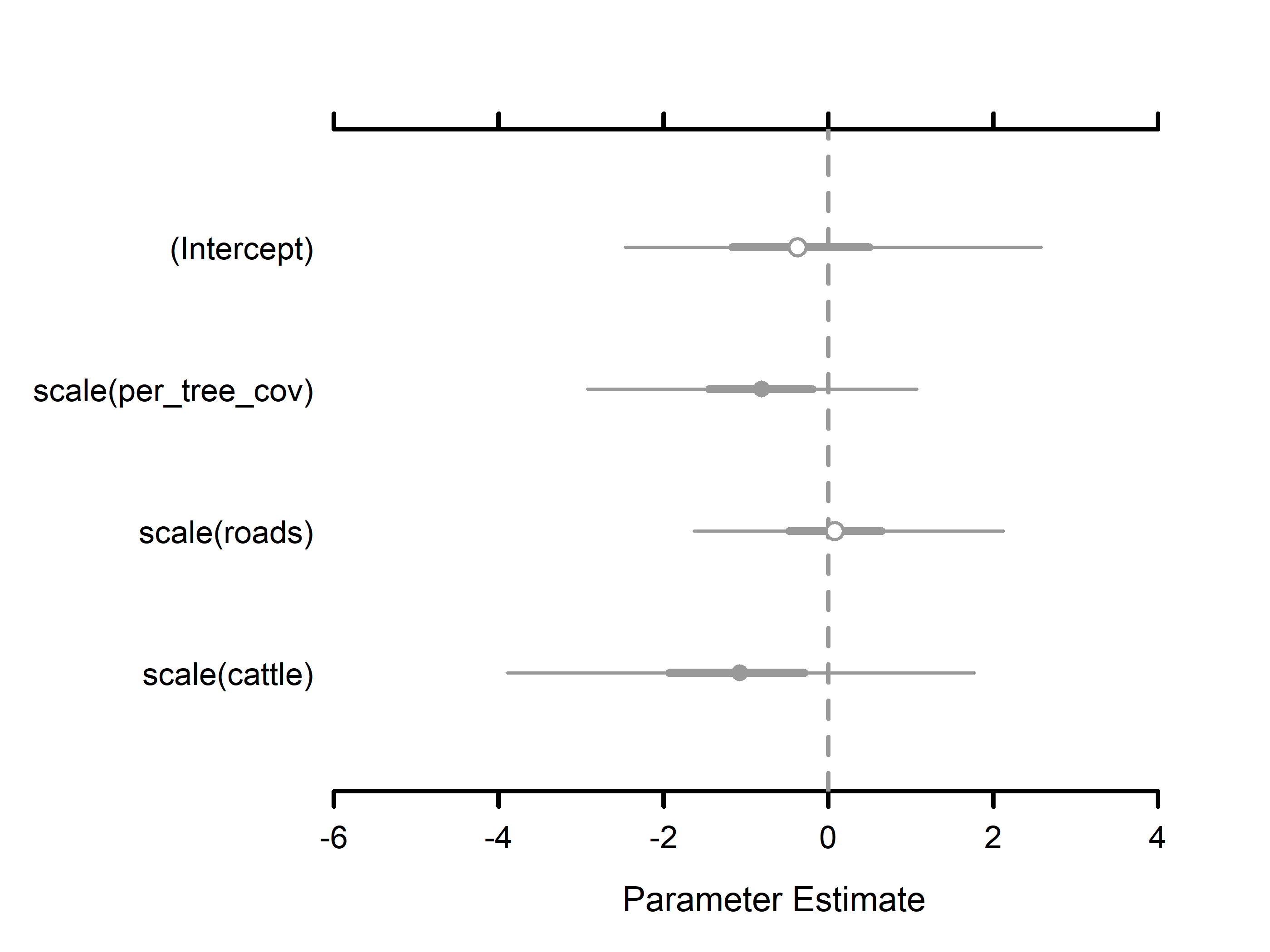
#> Occurrence (logit scale):
#> Mean SD 2.5% 50% 97.5% Rhat ESS
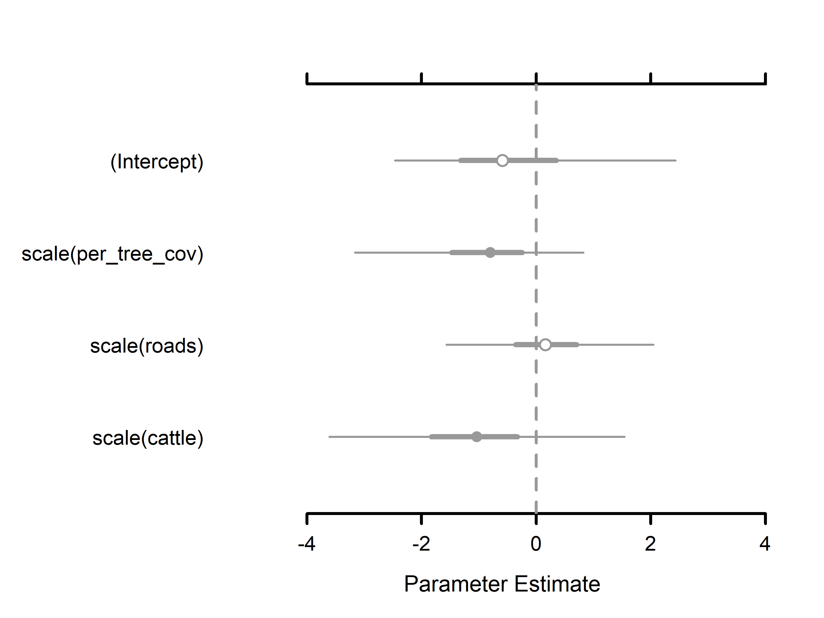
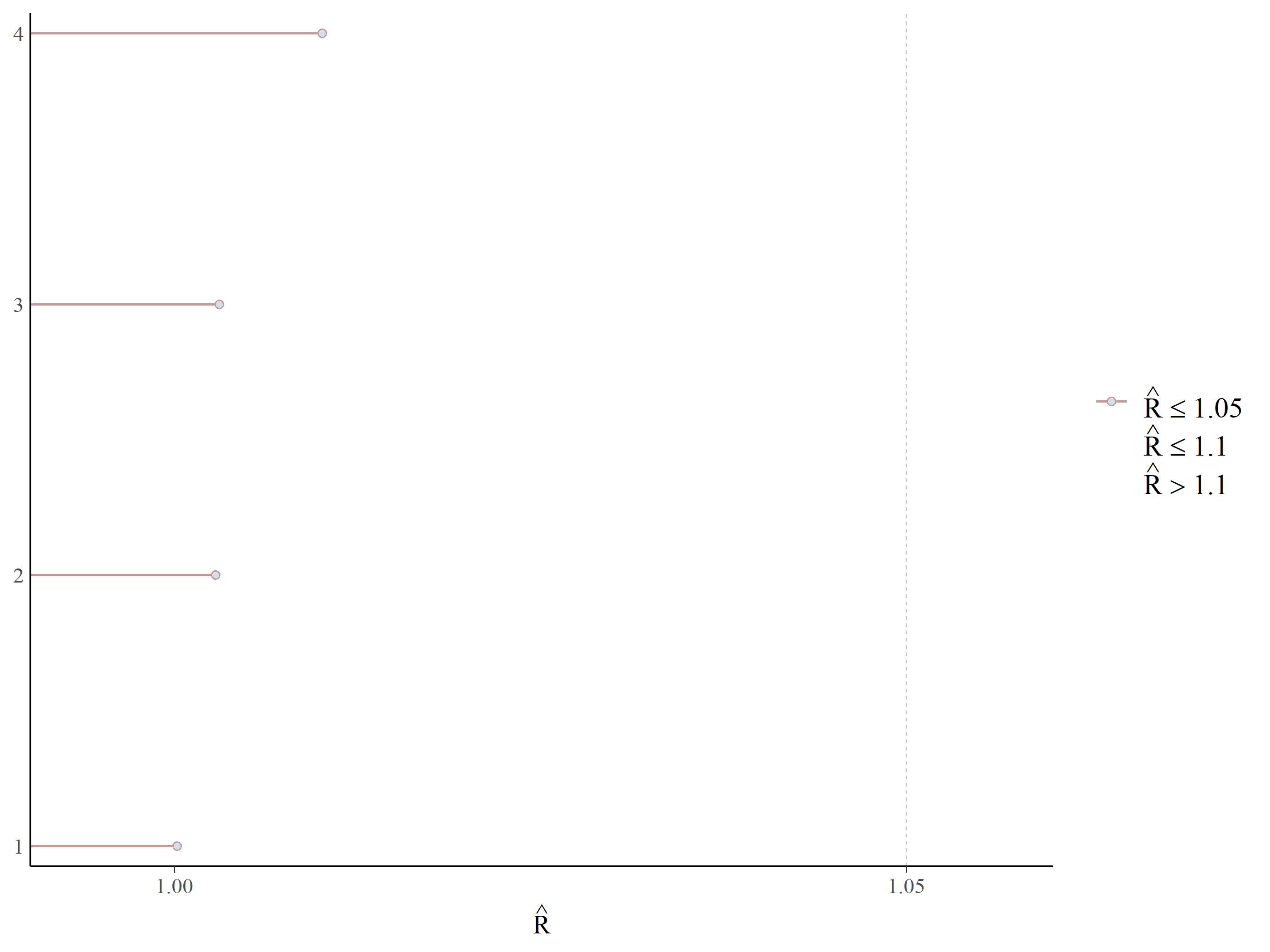
#> (Intercept) -0.2814 1.2412 -2.2262 -0.4676 2.5504 1.0004 4864
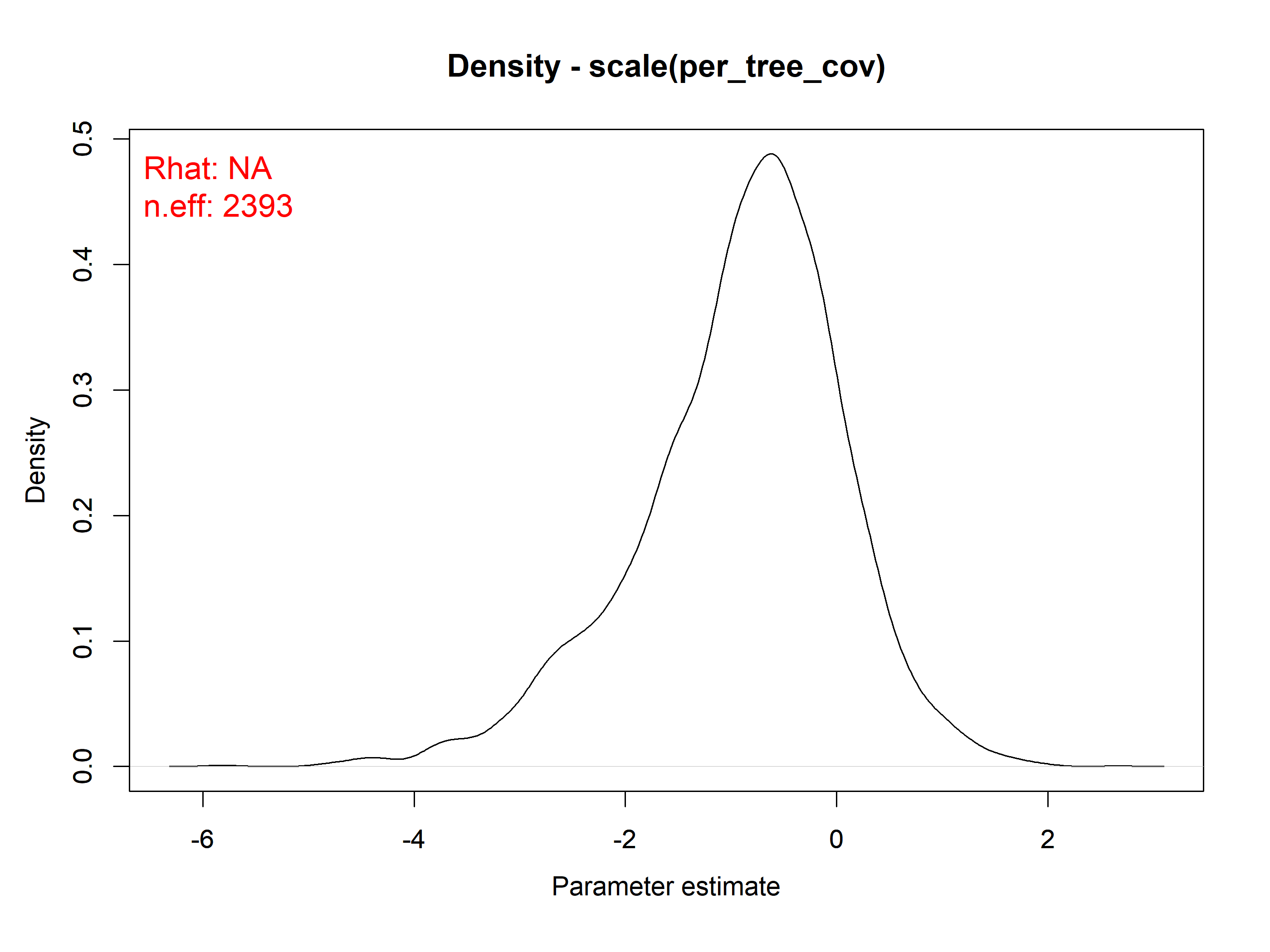
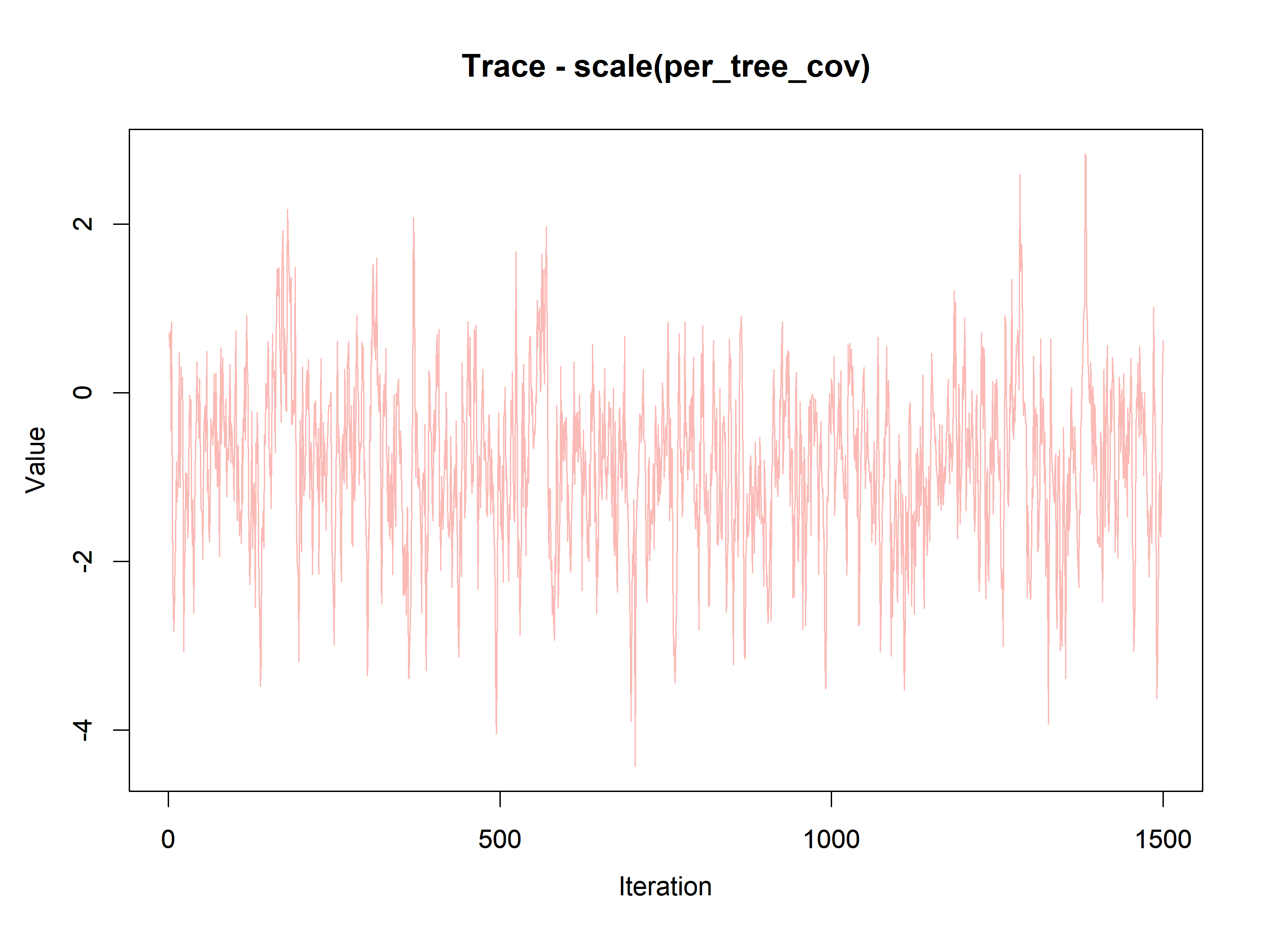
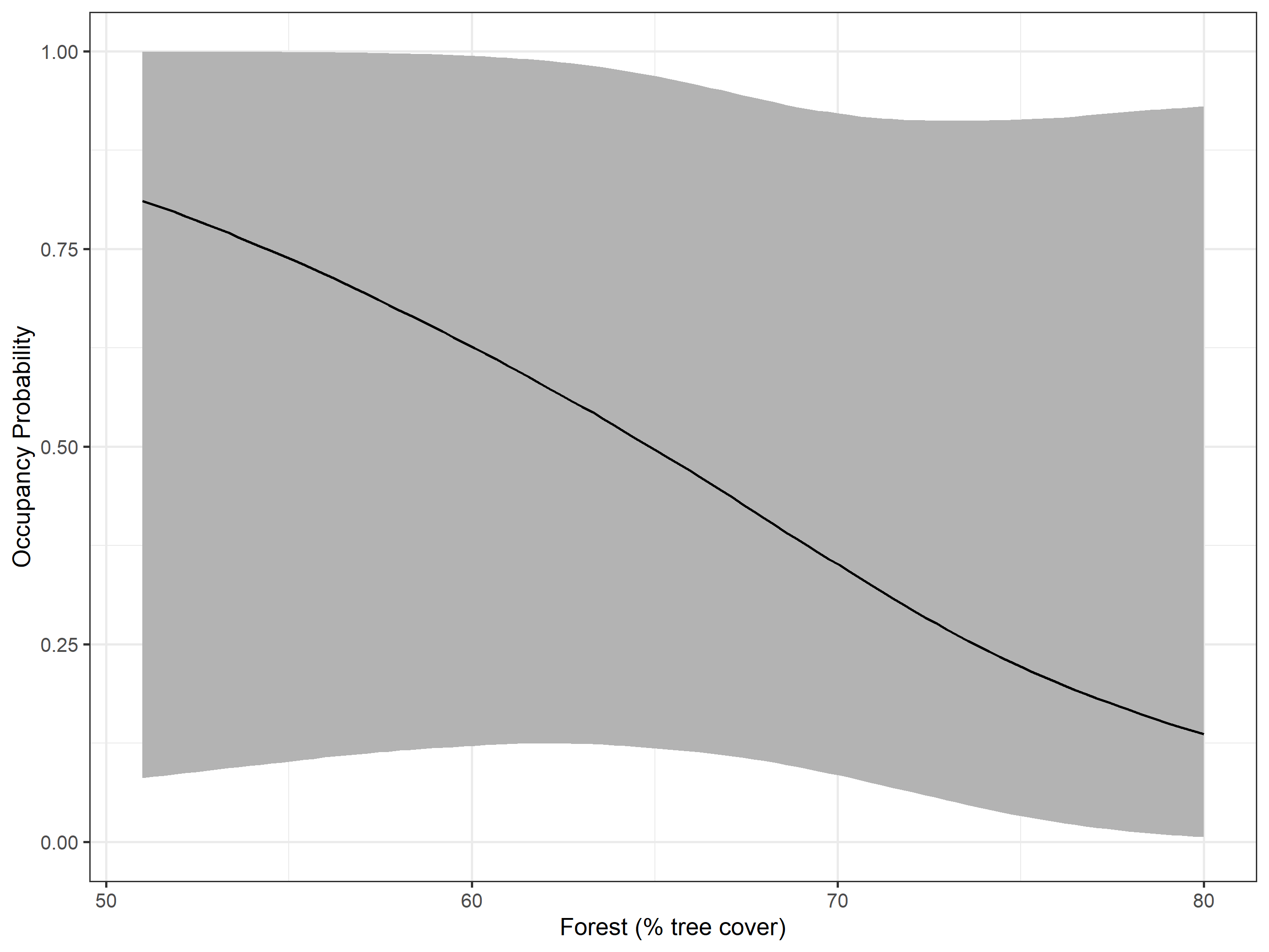
#> scale(per_tree_cov) -0.9001 0.9651 -3.1419 -0.7699 0.7196 1.0006 11358
#> scale(roads) 0.1314 0.8416 -1.5578 0.1258 1.8904 1.0004 14593
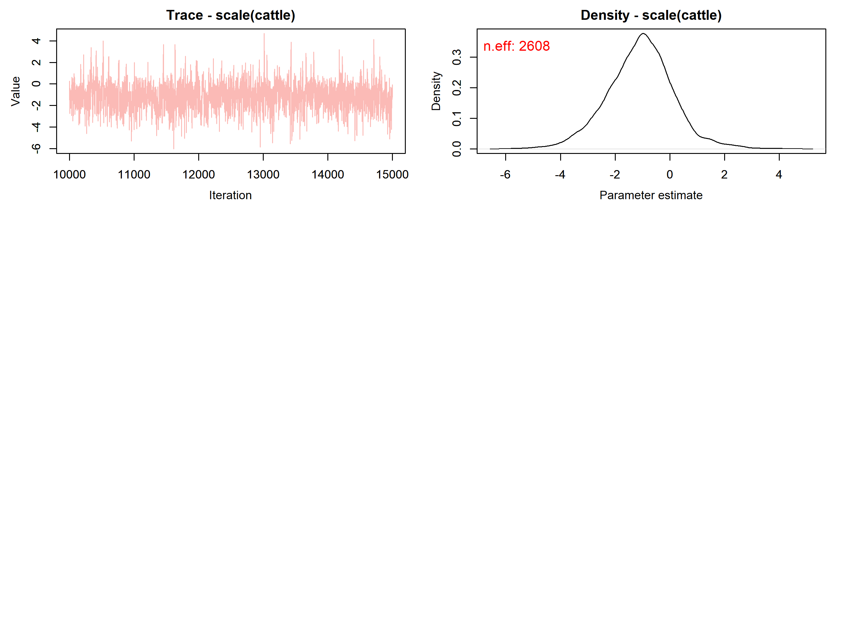
#> scale(cattle) -1.0808 1.2535 -3.5953 -1.0482 1.6156 1.0001 10296
#>
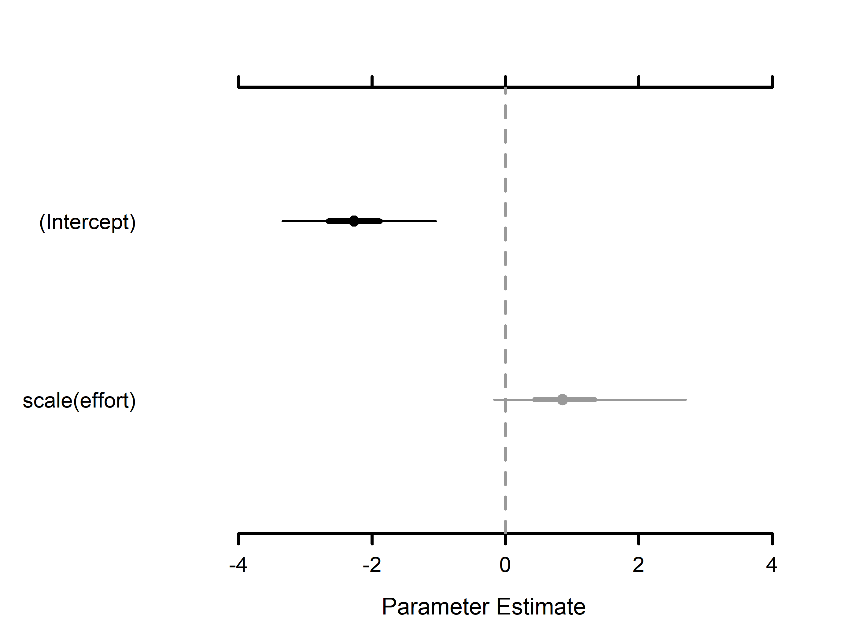
#> Detection (logit scale):
#> Mean SD 2.5% 50% 97.5% Rhat ESS
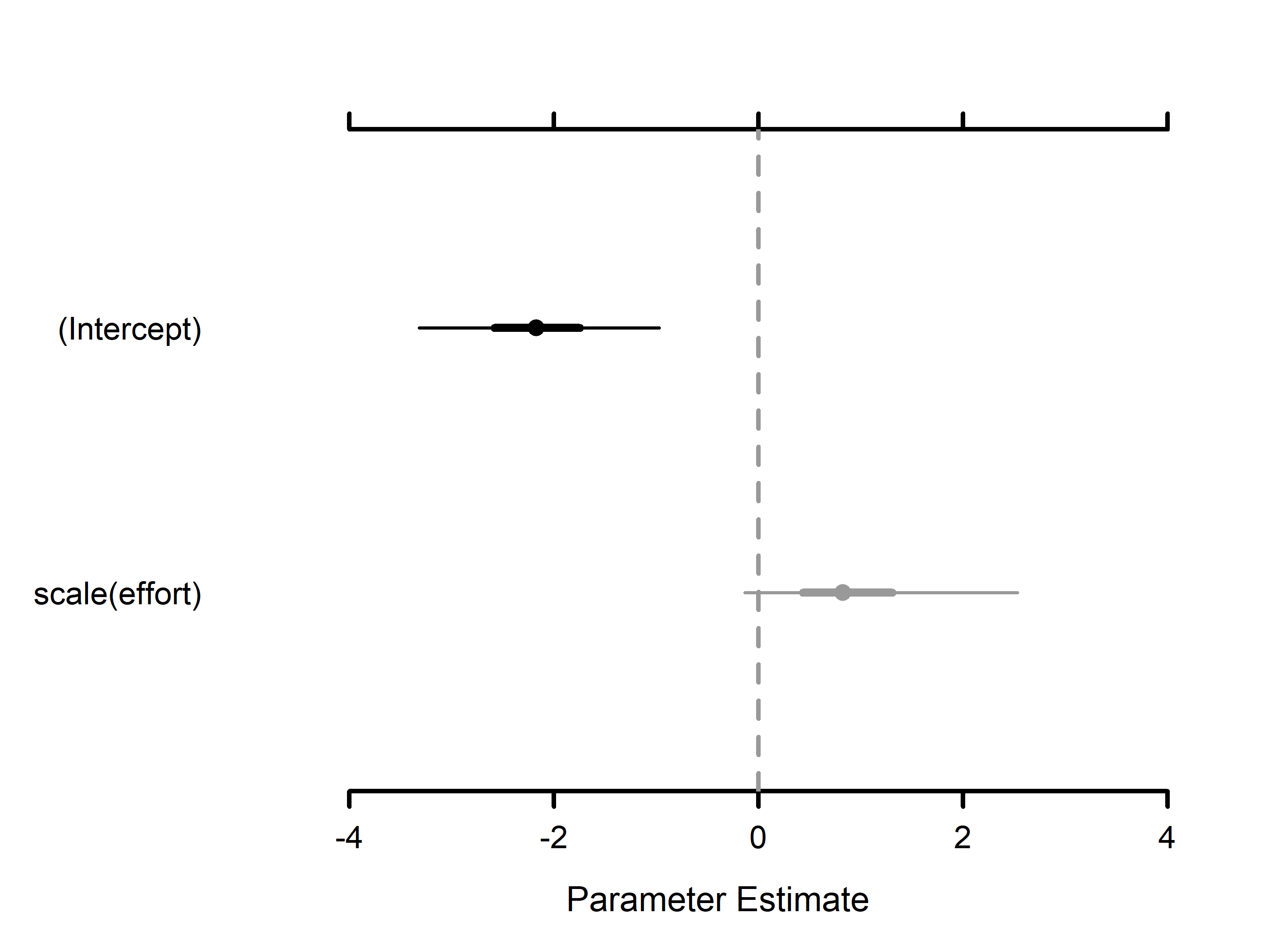
#> (Intercept) -2.1995 0.6168 -3.3787 -2.2150 -0.9882 1.0001 6851
#> scale(effort) 0.9347 0.6921 -0.1312 0.8343 2.5441 1.0006 15578