Graph of Sound Level Data from BirdNET-GO

Sound level from BirdNET-GO.

BirdNET-Go includes a powerful feature called Sound Level Monitoring. This is crucial for understanding the acoustic context of the environment, which helps in filtering unwanted noise and provides invaluable sounscape data for researchers.

The system registers sound levels in 1/3 octave bands, following the ISO 266 standard, providing a detailed frequency breakdown of the soundscape. The data is recorded as frequently as every ten seconds, offering continuous, advanced audio monitoring that gives a far richer picture of the overall soundscape than just a list of bird names. But I selected to get data each 30 seconds to have just two sound levels samples per minute.

Getting the data

In the past post, I explain more details about the sound levels and my custom solution.

At the end I have a CSV file that grows as fast as a Mega per day.

Plotting the data

To plot the sound levels I wrote the following R code:

library(readr)
library(tidyverse)
library(ggExtra)
library(viridis)
library(hms)

soundlevel_data <- read_csv("C:/Users/usuario/Downloads/soundlevel_data.csv", col_types = cols(timestamp = col_character()))

soundlevel_data$datetime <- ymd_hms(soundlevel_data$timestamp)
soundlevel_data$dia <- date(soundlevel_data$timestamp)
# Using lubridate to extract individual components and make hour
time_string <- as_hms(paste(hour(soundlevel_data$datetime),
                          minute(soundlevel_data$datetime),
                          second(soundlevel_data$datetime), sep = ":"))

soundlevel_data |> #filter(day(datetime)==c(22,23)) |> # filter one day
 ggplot(aes(x = time_string, y = frequency, fill = noise)) +
      geom_tile(height=.11) + # trick to remove white line
      # scale_fill_gradient(low = "yellow", high = "red") +
      scale_fill_viridis(option = "H") +
      scale_y_log10() +
      scale_x_time(date_breaks = "1 hour", date_labels = "%H")+
      facet_grid(rows = vars(dia)) +
      xlab("Hour") +
      ylab("Frequency (Hz)") +
        labs(fill = "Noise (dB)") +
   removeGrid() # + #ggExtra 
  # theme_classic() 

Here the graph

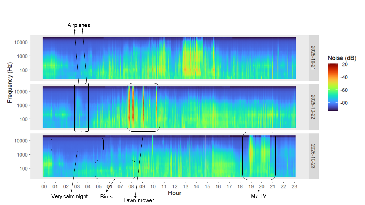
I tried to match the time with some acoustic events…

Why the sound levels are in negative scale?

In my BirdNET-GO data, the reference (0 dB) is set to the maximum possible level of the microphone (without distortion) that I use to capture the sound. In my case I am using a cheap MAONO USB Lavalier Microphone. It says is capable of recording at 192KHZ/24BIT and has an audio sensitivity of 30 Decibels. So -80 dB in the graph mean it is very quiet and 0 is very noisy, not real decibels. Perhaps I need to do some type of calibration here.

My readings range from about -45 dB to -89 dB, this suggests a relatively quiet environment (birds, ambient noise, and low noise). The higher frequencies (10-20 kHz) are much quieter (-80 to -89), which is normal for rural or natural soundscapes.

Why this scale is useful:

The logarithmic nature of the data matches how our ears perceive sound - a change of 10 dB is roughly perceived as “twice as loud.” So it also makes it easier to handle the huge range of sound intensities we encounter in the environment.

My sound level data is totally normal! The negative values just mean everything is related to the mic’s maximum capacity, which is good… or perhaps I need a much better mic?.

This work is licensed under a Creative Commons Attribution-ShareAlike 4.0 International License.