Chapter6 Occupancy analysis, ML method
Now that we have understood how the two processes work and interact; the ecological and the observational to produce the occupation data. After generating several data sets, now we only have to analyze them. The most direct and intuitive way is to use the occu function from the unmarked (Fiske & Chandler, 2011) package. Later we can use a Bayesian type model in the BUGS language to analyze the same data and in the end compare which of the two estimators, Maximum Likelihood or Bayesian, is closer to the true parameters.
6.0.1 Clearing R memory
Before we continue, and since we have already generated a large amount of data and models in the previous steps, we are going to clear the memory of R before we begin. We do this with the command:
rm(list = ls())Once we have done this we must re-run the code of the function that generates the data that we have created in Chapter 5.
After having loaded the function again we must return to
6.1 Generating the data
This time we will use a TEAM-type design (https://www.wildlifeinsights.org/team-network) with 60 sampling sites and 30 repeated visits, which is equivalent to the 30 days that the cameras remain active in the field. Again our species is the white-tailed tapir. For this example we will assume that detection is 0.6, occupancy is 0.8, and the interactions are much simpler with elevation as the only covariate explaining occupancy. However, for detection there is a more complex relationship, assuming that there is a slight interaction between the observation covariates. For observation, elevation and temperature interact with each other. Also, note how elevation influences in opposite directions with a positive sign at elevation for detection and negative for occupancy.
# Data generation
# Lets build a model were elevation explain occupancy and p has interactions
datos2<-data.fn(M = 60, J = 30, show.plot = FALSE,
                mean.occupancy = 0.8, beta1 = -1.5, beta2 = 0, beta3 = 0,
                mean.detection = 0.6, alpha1 = 2, alpha2 = 1, alpha3 = 1.5
                )

# Function to simulate occupancy measurements replicated at M sites during J occasions.
# Population closure is assumed for each site.
# Expected occurrence may be affected by elevation (elev),
# forest cover (forest) and their interaction.
# Expected detection probability may be affected by elevation,
# temperature (temp) and their interaction.
# Function arguments:
#     M: Number of spatial replicates (sites)
#     J: Number of temporal replicates (occasions)
#     mean.occupancy: Mean occurrence at value 0 of occurrence covariates
#     beta1: Main effect of elevation on occurrence
#     beta2: Main effect of forest cover on occurrence
#     beta3: Interaction effect on occurrence of elevation and forest cover
#     mean.detection: Mean detection prob. at value 0 of detection covariates
#     alpha1: Main effect of elevation on detection probability
#     alpha2: Main effect of temperature on detection probability
#     alpha3: Interaction effect on detection of elevation and temperature
#     show.plot: if TRUE, plots of the data will be displayed;
#               set to FALSE if you are running simulations.


#To make the objects inside the list directly accessible to R, without having to address
#them as data$C for instance, you can attach datos2 to the search path.

attach(datos2)         # Make objects inside of 'datos2' accessible directly

#Remember to detach the data after use, and in particular before attaching a new data
#object, because more than one data set attached in the search path will cause confusion.

# detach(datos2)         # Make clean up
6.2 Putting the data in unmarked
Unmarked is the R package we use to analyze the (Fiske & Chandler, 2011) occupancy data. To achieve this we must first prepare the data and collect it in an object of type unmarkedFrame. In this case we use the unmarkedFrameOccu function, which is specific for occupancy analysis of a single season or season. More about unmarked at: https://sites.google.com/site/unmarkedinfo/home
library(unmarked)
siteCovs <- as.data.frame(cbind(forest,elev)) # occupancy covariates
obselev<-matrix(rep(elev,J),ncol = J) # make elevation per observation
obsCovs <- list(temp= temp,elev=obselev) # detection covariates

# umf is the object joining observations (y), occupancy covariates (siteCovs)
# and detection covariates (obsCovs). Note that obsCovs should be a list of
# matrices or dataframes.

umf <- unmarkedFrameOccu(y = y, siteCovs = siteCovs, obsCovs = obsCovs)
The unmarked package allows us to graphically see how the data is arranged at the sampling sites with the plot function.
plot (umf)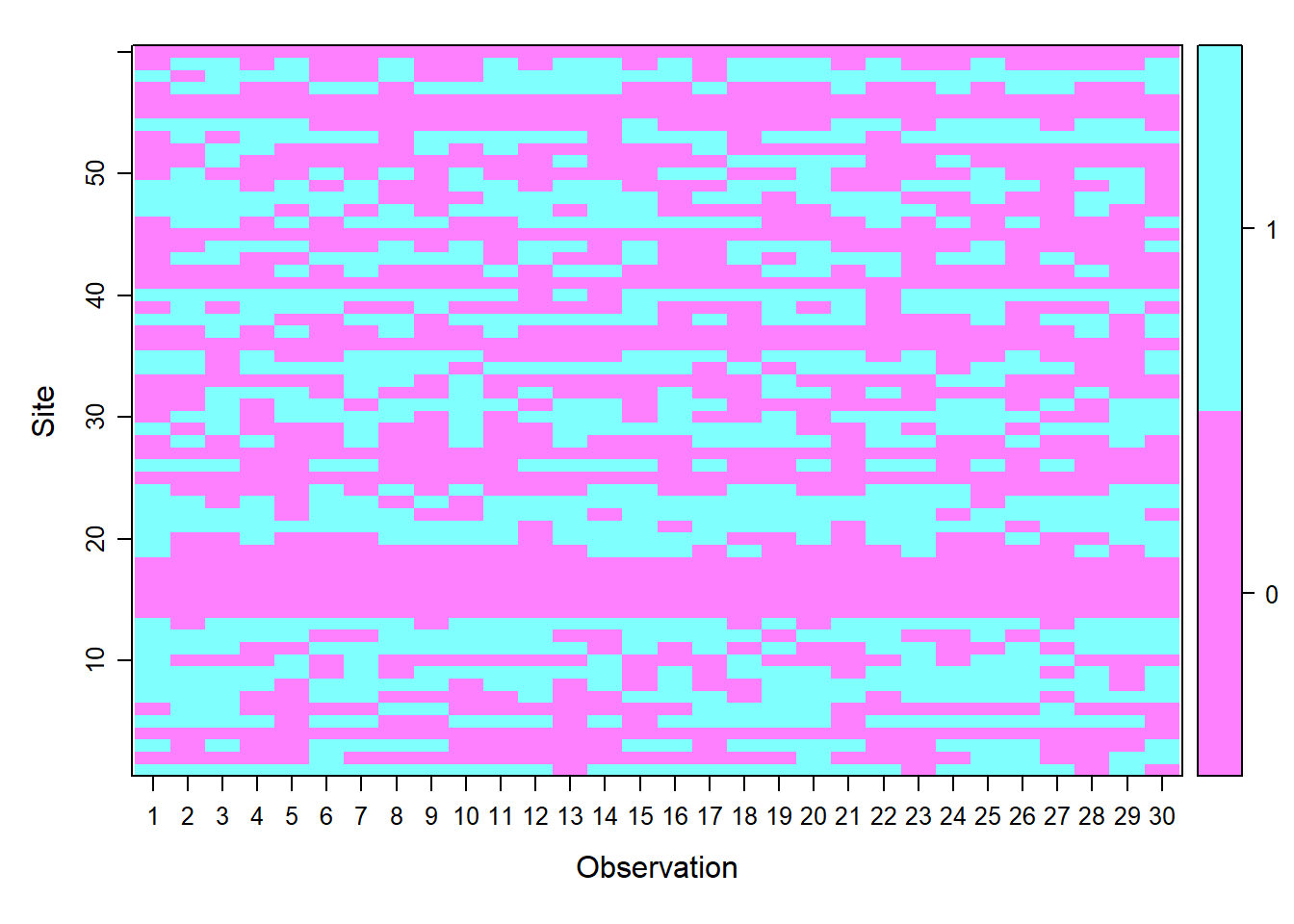
Figure 6.1: Inspección grafica del objeto umf.
6.3 Fitting the models
The next step is to fit the models that were required by varying the covariates. This is accomplished with the occu() function.
Keep in mind that in the model building process your models must have a biological meaning.
# detection first, occupancy next
fm0 <- occu(~1 ~1, umf) # Null model
fm1 <- occu(~ elev ~ 1, umf) # elev explaining detection
fm2 <- occu(~ elev ~ elev, umf) # elev explaining detection and occupancy
fm3 <- occu(~ temp ~ elev, umf)
fm4 <- occu(~ temp ~ forest, umf)
fm5 <- occu(~ elev + temp ~ 1, umf)
fm6 <- occu(~ elev + temp + elev:temp ~ 1, umf)
fm7 <- occu(~ elev + temp + elev:temp ~ elev, umf)
fm8 <- occu(~ elev + temp + elev:temp ~ forest, umf)
6.4 Model Selection
Unmarked allows you to perform a model selection procedure to select models based on the Akaike information Criterium (AIC) of each one. So the lowest AIC is the most parsimonious model according to our data (Burnham & Anderson, 2004).
models <- fitList( # here e put names to the models
  'p(.)psi(.)'                        = fm0,
  'p(elev)psi(.)'                     = fm1,
  'p(elev)psi(elev)'                  = fm2,
  'p(temp)psi(elev)'                  = fm3,
  'p(temp)psi(forest)'                = fm4,
  'p(temp+elev)psi(.)'                = fm5,
  'p(temp+elev+elev:temp)psi(.)'      = fm6,
  'p(temp+elev+elev:temp)psi(elev)'   = fm7,
  'p(temp+elev+elev:temp)psi(forest)' = fm8)

modSel(models) # model selection procedure
## nPars AIC
## p(temp+elev+elev:temp)psi(elev) 6 1630.77
## p(temp+elev+elev:temp)psi(.) 5 1636.27
## p(temp+elev+elev:temp)psi(forest) 6 1638.24
## p(temp+elev)psi(.) 4 1672.55
## p(elev)psi(elev) 4 1741.34
## p(elev)psi(.) 3 1746.83
## p(temp)psi(elev) 4 1898.56
## p(temp)psi(forest) 4 1906.03
## p(.)psi(.) 2 1969.25
## delta AICwt
## p(temp+elev+elev:temp)psi(elev) 0.00 9.2e-01
## p(temp+elev+elev:temp)psi(.) 5.49 5.9e-02
## p(temp+elev+elev:temp)psi(forest) 7.47 2.2e-02
## p(temp+elev)psi(.) 41.78 7.8e-10
## p(elev)psi(elev) 110.57 9.0e-25
## p(elev)psi(.) 116.06 5.8e-26
## p(temp)psi(elev) 267.79 6.5e-59
## p(temp)psi(forest) 275.26 1.6e-60
## p(.)psi(.) 338.48 2.9e-74
## cumltvWt
## p(temp+elev+elev:temp)psi(elev) 0.92
## p(temp+elev+elev:temp)psi(.) 0.98
## p(temp+elev+elev:temp)psi(forest) 1.00
## p(temp+elev)psi(.) 1.00
## p(elev)psi(elev) 1.00
## p(elev)psi(.) 1.00
## p(temp)psi(elev) 1.00
## p(temp)psi(forest) 1.00
## p(.)psi(.) 1.006.5 Prediction in graphs
The model with the lowest AIC can be used to predict expected results according to a new data set. For example, one might ask the expected abundance of deer at a higher elevation site. Predictions are also another way of presenting the results of an analysis. Here we will illustrate what the prediction of \(\psi\) and p looks like over the range of covariates studied. Note that we are using standardized covariates. If we were using covariates at their real scale, we would have to take into account that they have to be transformed using the mean and standard deviation.
Before using the model to predict it is a good idea to check the model parameters and their errors, then check graphically that the model fits well with the parboot function, which does a resampling of the model. This plot is interpreted as the model having a good fit, when the mean (dotted line) is between the intervals of the histogram. If the line is too far from the histogram the model might not be good at predicting.
summary(fm7) # see the model parameters##
## Call:
## occu(formula = ~elev + temp + elev:temp ~ elev, data = umf)
##
## Occupancy (logit-scale):
## Estimate SE z P(>|z|)
## (Intercept) 1.41 0.366 3.85 0.000117
## elev -1.63 0.656 -2.48 0.013082
##
## Detection (logit-scale):
## Estimate SE z P(>|z|)
## (Intercept) 0.53 0.0698 7.60 3.04e-14
## elev 1.80 0.1277 14.10 3.56e-45
## temp 1.16 0.1209 9.57 1.08e-21
## elev:temp 1.33 0.2211 6.00 1.96e-09
##
## AIC: 1630.771
## Number of sites: 60
## optim convergence code: 0
## optim iterations: 31
## Bootstrap iterations: 0pb <- parboot(fm7, nsim=250, report=10) # goodness of fit## t0 = 409.3793plot (pb) # plot goodness of fit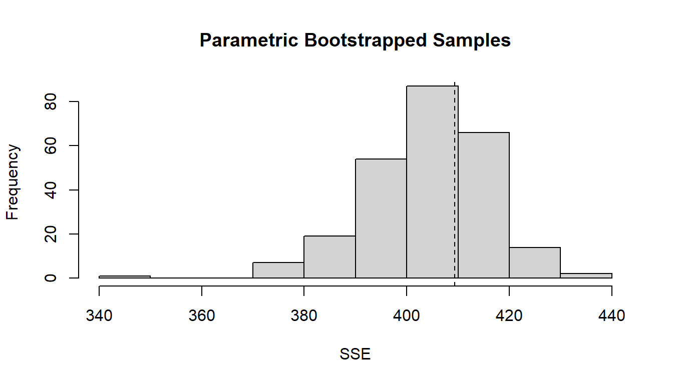
Figure 6.2: Graphical evaluation of the model fit fm7.
Now that we know that our best model has a good fit, we can use it to predict occupancy in the elevation range to see how it behaves on a graph.
elevrange<-data.frame(elev=seq(min(datos2$elev),max(datos2$elev),length=100)) # newdata
pred_psi <-predict(fm7,type="state",newdata=elevrange,appendData=TRUE)
plot(Predicted~elev, pred_psi,type="l",col="blue",
       xlab="elev",
       ylab="psi")
lines(lower~elev, pred_psi,type="l",col=gray(0.5))
lines(upper~elev, pred_psi,type="l",col=gray(0.5))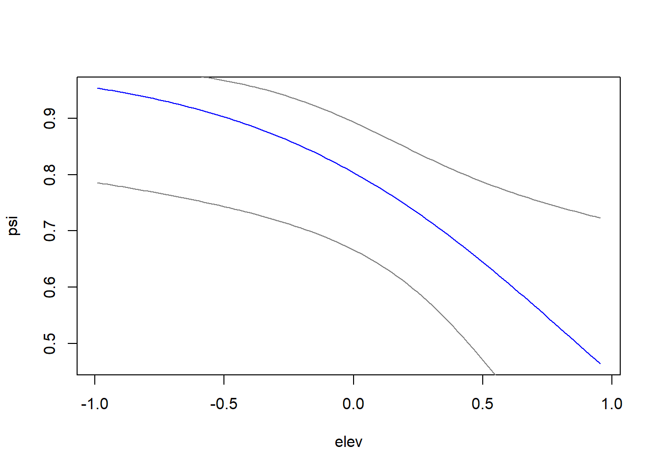
Figure 6.3: Plot of occupancy versus elevation.
6.6 Spatially explicit prediction
We can also use the best model to predict spatially explicitly if we have the maps. As an illustration we will construct simulated maps for each of our covariates. The maps arise from a random pattern of points with a Poisson distribution. We then convert these points to an interpolated surface.
# lets make random maps for the three covariates
library(raster)
library(spatstat)
set.seed(24) # Remove for random simulations

# CONSTRUCT ANALYSIS WINDOW USING THE FOLLOWING:
xrange=c(-2.5, 1002.5)
yrange=c(-2.5, 502.5)
window<-owin(xrange, yrange)

# Build maps from random points and interpole in same line
elev   <- density(rpoispp(lambda=0.6, win=window)) #
forest <- density(rpoispp(lambda=0.2, win=window)) #
temp   <- density(rpoispp(lambda=0.5, win=window)) #

# Convert covs to raster and Put in the same stack
mapdata.m<-stack(raster(elev),raster(forest), raster(temp))
names(mapdata.m)<- c("elev", "forest", "temp") # put names to raster

# lets plot the covs maps
plot(mapdata.m)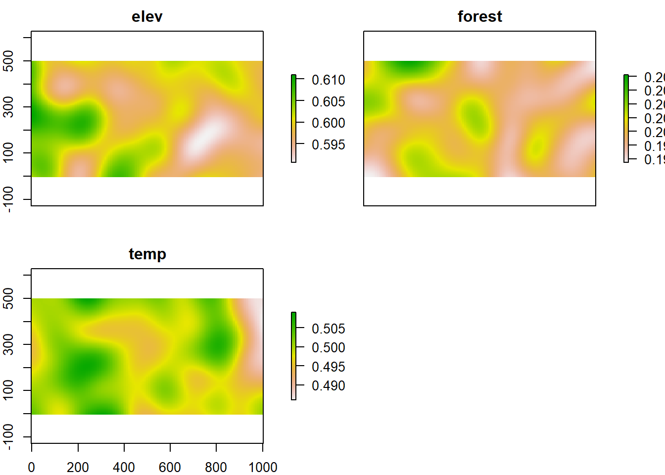
Figure 6.4: Simulated map of elevation, forest and temperature.
Once we have our covariate maps, we use them to predict with the best model. In this way we can have a map with predictions of the occupancy and the probability of detection.
# make the predictions
predictions_psi <- predict(fm7, type="state", newdata=mapdata.m) # predict psi
predictions_p   <- predict(fm7, type="det",   newdata=mapdata.m) # predict p
# put in the same stack
predmaps<-stack(predictions_psi$Predicted,predictions_p$Predicted)
names(predmaps)<-c("psi_predicted", "p_predicted") # put names
plot(predmaps)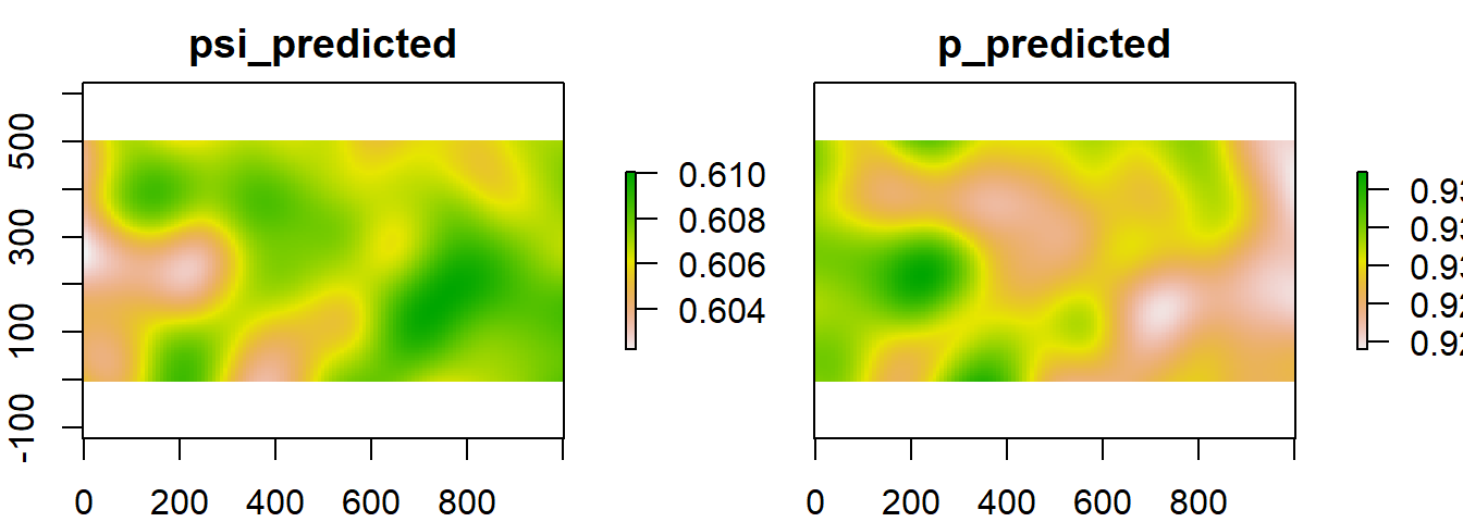
Figure 6.5: Spatially explicit detection and occupancy models.